If you have used Claude Code or Codex for more than a few sessions, you have probably noticed that first-turn pause. That brief hang before the agent does anything useful. I finally looked into why. Someone set up a proxy to count the tokens flowing between a coding agent and the API on each request. The number that came back was hard to believe. Before the agent had written a single line of code, before it had read a single file, it had already consumed 27,000 input tokens. On every single request.

The breakdown tells the story. System prompt: a few thousand tokens. Tool definitions: another several thousand. Memory files loaded at startup: more thousands. By the time the model saw the user’s actual task, over a quarter of a typical context budget was already spent on the agent talking to itself.

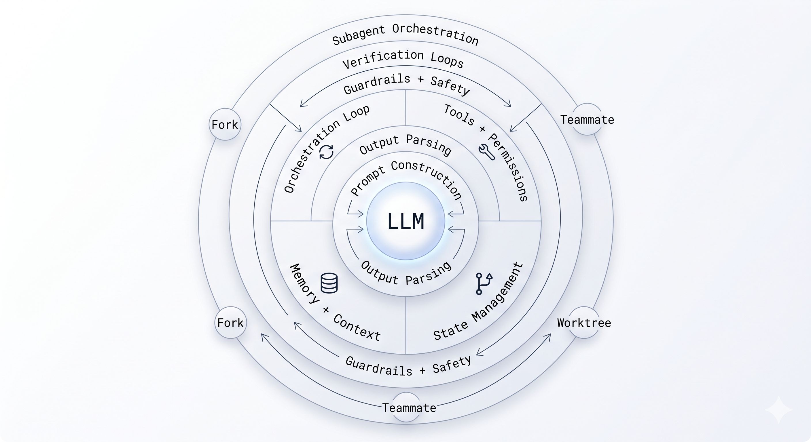
This is the central tension of building with LLMs today, and it has a name: the agent harness. The LangChain team put it cleanly: “If you’re not the model, you’re the harness.” Everything that wraps around the LLM to make it behave like an agent is the harness: the orchestration loop, the tools, the memory system, the context management, the state persistence, the error handling, the guardrails, the prompt assembly, the output parsing, the verification loops, the subagent coordination. The model is a component. The harness is the product.

The Von Neumann Analogy

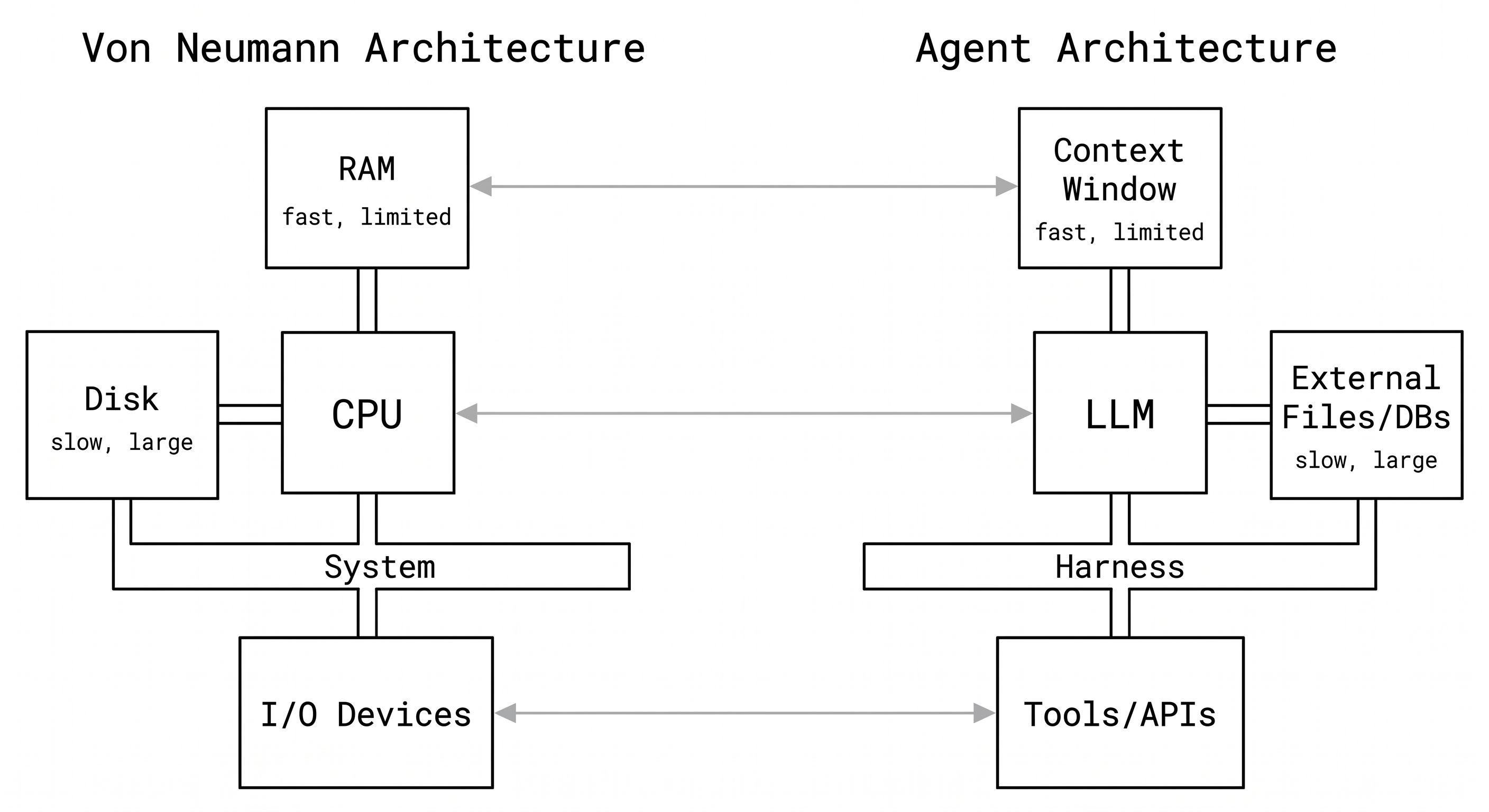
The best mental model for understanding a harness comes from computer architecture. A researcher framed it this way: a raw LLM is like a CPU with no RAM, no disk, and no I/O. Technically powerful. Practically useless on its own.

Map it out:

Every time you build an agent, you are reinventing the operating system. The orchestration loop is your scheduler. Context management is your memory manager. Tool execution is your I/O subsystem. Safety checks are your kernel-level permissions. These are not new problems. They are problems that OS designers solved in the 1970s and 1980s. The vocabulary has changed. The constraints are identical.

This is not a metaphor to be cute. It is a useful frame because it tells you what the hard problems actually are. Memory management in agents (what goes into the context window, when, and in what form) is as non-trivial as memory management in operating systems. Most of the bugs you will hit in production agent systems are not model bugs. They are OS bugs.

The Harness Tax

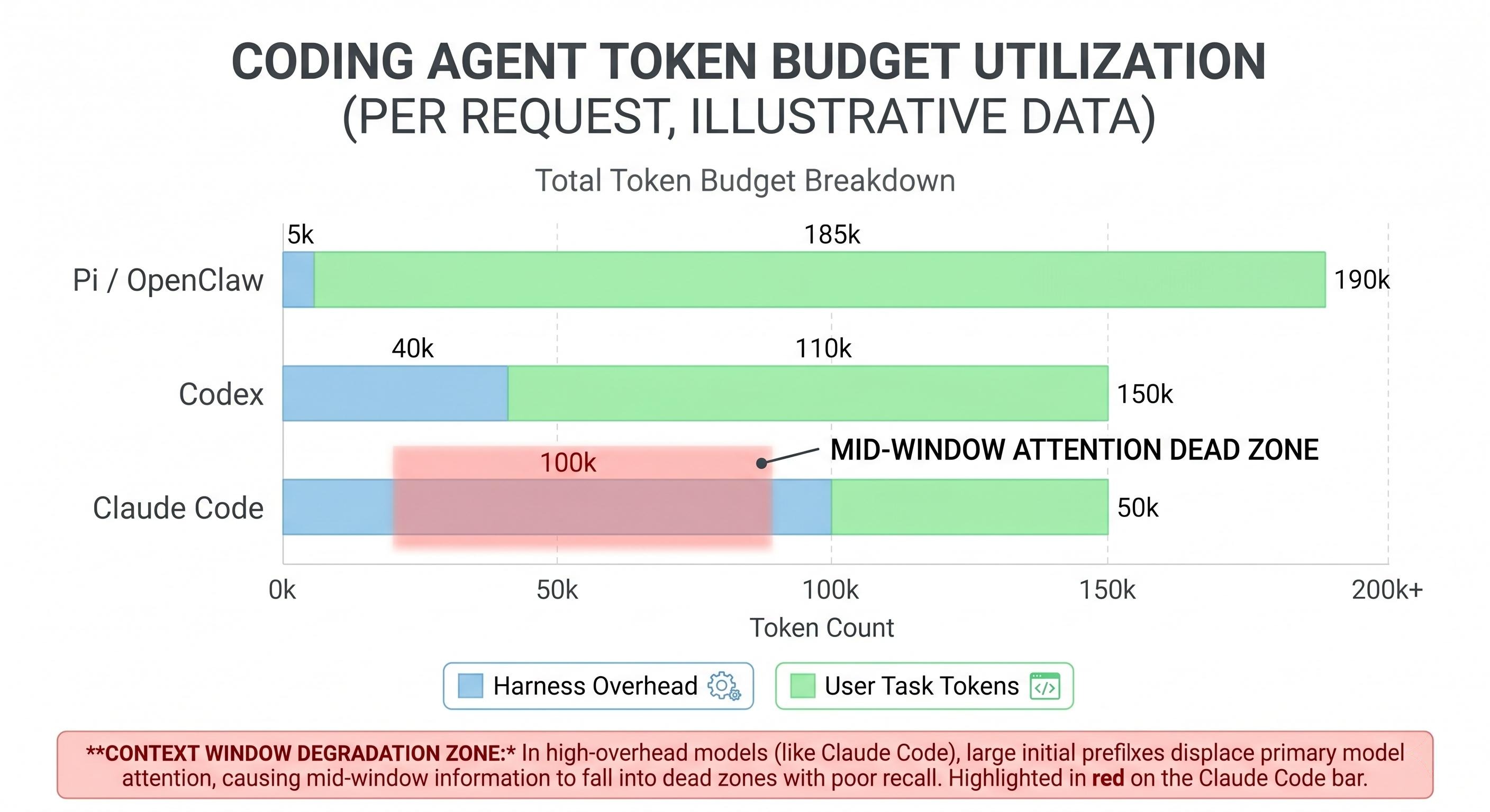
Every agent carries what I call the harness tax: the tokens the agent spends on itself before spending a single token on the user’s task. Someone benchmarked this directly across three coding agents running the same trivial task (write a Fibonacci script):

A 40-turn session at Claude Code’s rate burns roughly 1.12 million input tokens. About half of that is harness overhead. That is real money, and it is also a real engineering constraint. Claude Code ships around 24 tool definitions on every single request. In any given session, most of those tools never get called. But each tool schema takes up tokens, and those tokens sit in the context window the whole time.

This is where it stops being just a cost problem and becomes a quality problem. Token position matters. Research from Stanford’s “Lost in the Middle” paper showed model performance degrades 30%+ when key content lands in the middle of the context window rather than at the start or end. Every token of harness overhead is a token of displacement. When your agent’s context fills up with tool schemas for tools it will never use, those tokens are physically pushing your user’s code and intent toward that degraded middle zone.

I call it context rot. The harness bloats the context, the context degrades model attention, model attention degradation hurts the quality of the actual task. A thick harness can make your agent dumber, not smarter.

The design tension is real: more harness capabilities mean more tokens, and more tokens mean worse attention distribution. Every tool you add to your agent is a tradeoff between what it can do and how well it does everything else.

Anatomy of a Production Harness

Different practitioners slice the harness differently. One breakdown lists 12 components. An open-source mini coding agent uses 6. The territory is the same either way. Here is how I group it.

The Loop: Orchestration and State

Every agent harness has an orchestration loop at its core. You may know it as ReAct (Reasoning plus Acting) or the TAO cycle (Thought, Action, Observation). The structure is always the same:

1. Assemble the prompt (system instructions + tools + memory + conversation history + user message)
2. Call the LLM
3. Parse the output: is it a final answer, a tool call, or a handoff to another agent?
4. If tool call: validate inputs, check permissions, execute in sandbox, capture output
5. Package tool results as new messages
6. Update context, trigger compaction if needed
7. Loop back to step 1

Anthropic’s Claude Agent SDK describes their implementation as a “dumb loop where all intelligence lives in the model.” That is the right way to think about it. The loop is plumbing. It should be boring.

State management is the part that gets complicated. How does an agent resume after a context window fills? Claude Code uses git commits as checkpoints. Long-running tasks use progress files as scratchpads, and the filesystem provides continuity across context windows. LangGraph uses typed dictionaries with explicit checkpoint snapshots.

Error handling in agents is sneaky. A 10-step task with 99% per-step success has only 90.4% end-to-end success. There are four failure types worth designing for: transient failures (retry), LLM-recoverable failures (the model can self-correct), user-fixable failures (stop and ask), and unexpected failures (fail loudly and log everything). Most agent failures in production are compound failures where the root cause is two steps back.

Tools and Prompt Construction

Tools are how the agent reaches outside the context window. Each tool is a schema (name, description, input parameters, output format) injected into the prompt on every request. The harness handles registration, input validation, permission checking, sandboxed execution, and result capture.

Claude Code gates around 40 discrete tool capabilities independently. The permission model is three-staged: trust establishment (who is asking and in what context), permission check (is this action allowed for this trust level), and explicit user confirmation for high-impact operations.

Prompt construction is more nuanced than most people realize. The hierarchical assembly order matters: system prompt, tool definitions, memory files, conversation history, current user message. Changing that order changes model behavior.

The key optimization here is splitting your prompt into a stable prefix and a changing suffix. The stable prefix (system instructions, tool definitions, workspace summary) rarely changes within a session. The changing suffix (recent conversation, memory notes, current task) updates every turn. Why does this split matter? Because of prompt caching.

Anthropic’s API lets you mark cache breakpoints on content blocks using cache_control. Everything from the start of the request up to that breakpoint gets cached server-side with a 5-minute TTL. Cache reads cost roughly 10% of normal input token pricing. Cache writes (the first time) cost 25% more. After that first call, every subsequent turn within the TTL window gets the prefix at a 90% discount.

Here is how an open-source coding agent (mini-coding-agent) structures this in practice:

def build_prefix(workspace_context):
    """Stable portion of the prompt. Cached across turns."""
    return {
        "role": "system",
        "content": [
            {"type": "text", "text": AGENT_INSTRUCTIONS},
            {"type": "text", "text": workspace_context.summary()},
            {"type": "text", "text": tool_descriptions(),
             "cache_control": {"type": "ephemeral"}}  # <-- cache breakpoint
        ]
    }

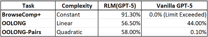
def build_prompt(prefix, memory_notes, history, user_message):
    """Combines cached prefix with per-turn changing suffix."""
    return [prefix] + memory_notes + history + [
        {"role": "user", "content": user_message}
    ]

The build_prefix function assembles the agent instructions, a workspace summary (git branch, repo root, project docs), and tool descriptions into a single block with a cache breakpoint at the end. Everything after that breakpoint (memory, transcript, user message) is the changing suffix that gets processed at full price each turn.

Claude Code follows the same principle but at a much larger scale. Its stable prefix runs about 27,000 tokens (system prompt + 24-40 tool schemas + memory index files). The math on caching that prefix is significant:

Without caching: 40-turn session x 27k prefix = 1,080,000 prefix tokens at full price

With caching: first turn pays 1.25x write cost on 27k tokens, remaining 39 turns pay 0.1x read cost

Result: roughly 87% savings on the stable prefix portion alone

The 5-minute TTL resets on each cache hit, so as long as the agent makes at least one API call every few minutes (which is typical in interactive coding sessions), the cache stays warm. The tradeoff is architectural: anything you put in the prefix must be truly stable. If you change even one token in the cached block, the entire cache invalidates and you pay the full write cost again. This is one reason Claude Code loads memory files in a specific order and keeps tool definitions static across turns.

Output parsing is where most brittle failures live. With native tool calling (structured tool_calls objects), you bypass a lot of free-text parsing pain. Before tool use was standardized, agents had to parse structured output out of prose, and models would use slightly different formats, omit fields, or add extra text. The lesson from Claude Code’s build of the AskUserQuestion tool: even a well-designed tool fails if the model does not understand when to call it. Tool design is as much about the model’s training distribution as it is about the schema.

Memory and Context

Memory in agents has two layers.

Short-term memory is the conversation history in the context window. It is fast and immediately available. It is also expensive and finite.

Long-term memory is everything that persists beyond a single context window. This includes project-level knowledge files (CLAUDE.md, AGENTS.md), session transcripts, task histories, user preferences. Claude Code uses a three-tier approach: a lightweight index file (150 characters max per entry, always loaded), detailed topic files loaded on demand, and raw transcripts used only for search.

The LangChain team makes a point worth sitting with: memory is not a module you plug into an agent harness. The team at Letta put it this way: “Asking to plug memory into an agent harness is like asking to plug driving into a car.” The harness controls what gets loaded into context, what survives compaction, how the filesystem is exposed, and how metadata is presented. Memory and harness are deeply coupled. You cannot really separate them.

The implication is uncomfortable: if your memory lives inside a closed harness (OpenAI’s Responses API with server-side compaction, Anthropic’s Managed Agents), you do not own your agent’s accumulated knowledge. Switching models means losing threads. This is not an accident. Model providers have strong incentives to lock users in via memory, because model switching costs are near zero today, but agent switching costs (accumulated state, learned preferences, project context) are high.

Context management is the harness’s most active responsibility during a long task:

• Compaction: when context fills, summarize old turns into a dense representation and drop the originals
• Observation masking: verbose tool outputs (like a full file listing) get hidden from the active window after their immediate turn
• Just-in-time retrieval: instead of loading all memory files at startup, load only what is relevant to the current task
• Subagent delegation: offload context-heavy subtasks to subagents that run in their own context windows and return only 1,000-2,000 token summaries

The right approach is to keep recent events rich while compressing older events aggressively. Recent context is almost always more relevant. Old context can usually be summarized or dropped.

Guardrails and Verification

Verification loops are the highest-ROI investment in a production harness. The Claude Code team measured a 2-3x quality improvement from adding verification. There are three levels:

1. Rules-based: run tests, linters, type checkers after each change. Fast and deterministic.
2. Visual: take a screenshot and confirm the UI looks correct. Works for frontend work where tests do not tell the full story.
3. LLM-as-judge: have a separate model review the output for correctness, completeness, or policy compliance. Expensive but catches things rules miss.

Subagent orchestration lets a harness parallelize work across multiple agent instances. Claude Code supports three patterns:

• Fork: a byte-identical copy of the current agent context, for truly parallel independent tasks
• Teammate: a separate agent in its own terminal pane with a file-based mailbox for coordination
• Worktree: an agent with its own git worktree and isolated branch, for tasks that need to diverge from the main codebase without interference

Thin Harness, Fat Skills

Here is a principle that surprised me when I first encountered it: giving your agent fewer tools often makes it better.

Pi (the reasoning engine behind OpenClaw) uses exactly four tools: read file, write file, edit file, and shell command. That is it. The reasoning is straightforward. Models trained on millions of GitHub repos and shell sessions already know how to use grep, find, ls, git log, and a thousand other utilities. If you want to search files, you do not need a search_files tool. You can just run grep -r. The tool schema would consume tokens to define something the model can already do with a shell command. Thin harness, fat skills.

The evidence from model evolution makes this trend concrete. Community benchmarks tracked harness changes across three Claude model generations:

• Sonnet 4.5: the harness needed explicit context reset mechanisms. When the model sensed it was running out of context, the harness would trigger a structured wrap-up and restart.
• Opus 4.5: the model handled context pressure better on its own. The explicit reset logic became unnecessary. It got removed.
• Opus 4.6: the harness had been doing sprint decomposition, breaking large tasks into smaller subtasks with explicit planning steps. With Opus 4.6, removing that entirely improved performance. The model planned better without the scaffolding.

Three model generations. Three layers of harness removed. What was load-bearing infrastructure in January was dead weight by March.

Manus (another coding agent) rebuilt their entire harness five times in six months. Each rebuild removed complexity. The team at Vercel reportedly removed 80% of the tools from v0 and got better results. Claude Code achieves 95% context reduction in some configurations via lazy loading: tools and context loaded only when needed, not upfront.

The pattern is consistent: as models improve, the complexity that compensates for their limitations becomes unnecessary. Harness code is temporary by nature. If you are writing harness logic that feels permanent, you are probably compensating for a model limitation that will be trained away within a generation or two.

There is a real tension here though. The “thin harness” principle applies to general-purpose capabilities. Task-specific harnesses tell a different story. One practitioner reported a +16 percentage point improvement by replacing a generic agent setup with a harness engineered specifically for financial data tasks. Generic harnesses give you acceptable performance across many tasks. Task-specific harnesses give you significantly better performance on the tasks that matter. Models are also “non-fungible in their harness”: dropping Codex into the Claude Code harness produces poor results because models are post-trained with specific harness assumptions baked in. The harness and the model form a unit.

The Meta-Harness

The most interesting recent development in this space is work coming out of Stanford: automated harness optimization.

The setup is a five-step loop:

1. Inspect: an LLM agent searches the filesystem for previous task results and execution traces
2. Diagnose: it reasons about what failure modes the traces reveal
3. Propose: it writes new harness code, typically a single-file Python change
4. Evaluate: run the modified harness on a task distribution, record the reward
5. Update: push results back to the filesystem, loop

They used Claude Code as the proposer agent. After enough iterations of this loop, the automated system hit 76.4% pass rate on TerminalBench, surpassing hand-designed harnesses. The key finding: the system needs unrestricted access to all previous experiment history. Text optimization loops that only see reward scores and summaries underperform badly. The dependencies are long-horizon. You need the full trace to diagnose the root cause.

This connects to a concept researchers describe as the model-harness training loop: what the harness does today gets trained into the model tomorrow. Anthropic observes which harness primitives are most effective in production, and subsequent model versions are post-trained to be better at using them natively. Then the harness can shed that layer and push to the next frontier. The harness is, in a real sense, the model’s training data pipeline for the next generation.

The business dimension matters too. Agent framework developers have pointed out that model providers are strongly incentivized to build lock-in at the harness layer, specifically through memory. OpenAI generates encrypted compaction summaries that cannot be used outside their ecosystem. Anthropic’s Claude Managed Agents puts the entire agent runtime behind an API. Switching the underlying model is nearly free today. Switching the harness, with all the accumulated memory and learned preferences it holds, is not.

If you do not own your harness, you do not own your agent.

Closing Thoughts

The thing I keep coming back to is how much engineering surface area lives outside the model. When an agent fails in production, the first instinct is to blame the LLM. Usually the problem is elsewhere: a tool schema that ambiguously describes when a tool should be called, a compaction strategy that lost a key piece of project context, a verification loop that was never implemented, an error type that was not classified and got silently swallowed.

A few principles that have crystallized for me after going deep on this:

Measure your harness tax first. Before optimizing anything else, count the tokens your agent spends before the user’s task begins. You may be surprised. Many teams have never looked at this number.

Build for removal. Every piece of harness logic should have a mental annotation: “this becomes unnecessary when the model can do X natively.” When that model generation ships, delete the code. Treat harness complexity as technical debt with a known expiration date.

Invest in verification loops. The data is consistent: 2-3x quality improvement from good verification, for relatively low implementation cost. Rules-based verification (linters, tests, type checkers) is the easiest starting point and often sufficient for 80% of the quality gain.

Be deliberate about memory architecture. Memory is the stickiest part of the stack. The decisions you make about where memory lives and in what format determine what vendor you are locked into and how much of your agent’s accumulated knowledge you actually own. Design this intentionally, not by accident.

The harness is where most of the interesting engineering in agentic AI lives right now. The model is improving fast. The harness is where the real systems thinking happens. And as the LangChain team put it: if you’re not the model, you’re the harness.

Running a frontier-tier model locally now takes only two commands—a significant shift from the complex setups required just a year ago.

On April 2, 2026, Google DeepMind released Gemma 4, a family of open-weight models distilled from Gemini 3. These models are designed to run on consumer hardware, reaching performance parity with models like GPT-5-mini on coding benchmarks, while offering native multimodal support for images and audio. Crucially, the release uses the Apache 2.0 license, enabling unrestricted commercial deployment. Following its launch, the consensus across developer communities is that this is a milestone release, though it comes with specific architectural trade-offs.

What Is Gemma 4?

Gemma 4 is a family of four models ranging from an edge-optimized 2B-class system to a 31B dense model that competes with closed-source frontier models. Every variant is trained on over 140 languages, and features a common architectural core with per-model specializations.

Three key factors define this release:

• Apache 2.0 Licensing: Previous Gemma models utilized a custom license that created ambiguity for certain commercial agentic systems. Gemma 4 is fully Apache 2.0, allowing users to modify, deploy, and build products without restriction.
• Multimodal Input: All four models can process text and images. The two “Edge” variants (E2B and E4B) also support native audio input. Context windows reach up to 256K tokens for the larger models and 128K tokens for the edge variants.
• Local Inference Performance: The 26B Mixture of Experts (MoE) variant can achieve speeds of approximately 120–150 tokens/second on an RTX 4090 and up to 400 tokens/second on M5 MacBook Pro systems, thanks to its low active parameter count (~3.8B) during inference.

Note: Gemma 4 is an input-multimodal model; it processes text, images, and audio but outputs only text.

The Model Lineup; Pick Your Fighter

Gemma 4 ships in four variants. Understanding the naming is critical because Google’s choices here generated genuine controversy.

HuggingFace model cards:

• E2B: google/gemma-4-e2b-it
• E4B: google/gemma-4-e4b-it
• 26B-A4B: google/gemma-4-26B-A4B-it
• 31B: google/gemma-4-31b-it

The “E” Naming Controversy

The “E” in E2B and E4B stands for Effective parameters; the compute budget during a forward pass, not the weight count. E4B runs like a 4B model computationally, but it has 8 billion weights sitting in RAM. You are not saving memory. You are saving compute.

“E4B is 8B weights marketed as 4B… classic bait and switch.” Multiple Hacker News users echoed this. The practical impact: if you’re GPU-constrained at 8GB VRAM, E4B fits (barely). But if you expected Raspberry Pi-level memory footprints from E2B based on the name, you’d be disappointed.

The naming logic is internally consistent; “effective” accurately describes the computational budget, not the storage cost; but it inverts the intuition most people have from model naming conventions where the number refers to parameters in memory.

Also notable: there is no 12B model. When a Gemma team member (canyon289) was asked about this on Hacker News, they acknowledged the gap but didn’t explain it. E4B appears to be the intended replacement for the 12B niche, though its benchmark performance sits meaningfully below what a 12B dense model would achieve.

Architecture Deep Dive

Gemma 4’s architecture is more interesting than it first appears. This section covers the seven innovations worth understanding.

Attention: Local and Global, Interleaved

Every Gemma 4 model alternates between two types of attention layers:

• Local (Sliding Window) Attention: each token only attends to the nearest N tokens within a sliding window. Efficient, O(n×w) complexity.
• Global Attention: full attention over the entire context. Expensive, O(n²) complexity, but necessary for long-range coherence.

The ratio:

• E2B: 4 local : 1 global
• E4B, 26B-A4B, 31B: 5 local : 1 global

Sliding window sizes: 512 tokens for E2B/E4B, 1024 tokens for the larger variants.

Key change from Gemma 3: The last layer of every Gemma 4 model is always a global attention layer. Gemma 3’s 4B model had a local attention layer as its final layer, which created a bottleneck for tasks requiring full-sequence summarization. That’s fixed.

Why does this matter? For a 256K token context, you’d be doing global attention only once every 5 or 6 layers; most of the compute stays cheap. The local layers do the heavy lifting for nearby relationships; the global layers integrate across the full context.

The Global Attention Efficiency Trio

Running global attention over 256K tokens naively would be prohibitively expensive. Gemma 4 applies three orthogonal optimizations to global attention layers specifically. Together they make long-context global attention fast enough to be practical.

Grouped Query Attention (GQA)

Standard multi-head attention has one Key and one Value per Query head, so the KV cache scales linearly with the number of heads. GQA groups multiple Query heads to share a single KV pair.

Gemma 4’s grouping is asymmetric:

• Local attention: 2 Query heads per KV head (modest grouping, fine at local scale)
• Global attention: 8 Query heads per KV head (aggressive grouping, critical for long contexts)

To compensate for the information loss from aggressive grouping, the Key dimensions are doubled in global attention layers. More information per KV pair, fewer KV pairs total.

Key-Value Tying (K=V)

Applied only in global attention layers of the 31B and 26B-A4B variants. Instead of learning separate Key and Value projections, the model sets Keys equal to Values: K = V.

This means the model only needs to store one set of vectors for global attention layers instead of two; effectively halving the KV cache for those layers. A separate RMSNorm is applied to the projection for Keys vs. Values even when they’re tied, which preserves the ability to apply different normalizations to the same underlying vectors.

The practical effect: the “KV cache” for global attention layers becomes a “K-cache only”; a meaningful memory reduction at long contexts where global layer KV contributions would otherwise dominate.

p-RoPE: Partial Rotary Positional Encoding

Standard RoPE (Rotary Positional Encoding) applies a rotation to every pair of dimensions in the attention head to encode position. At very long contexts, the lower-frequency rotation pairs accumulate noise; small rotations compound across 256K positions into drift that corrupts semantic information.

Gemma 4’s solution: only rotate the first 25% of dimension pairs (p=0.25). The other 75% have their rotations zeroed out entirely. Those high-frequency pairs preserve their semantic content without positional noise accumulation, while the 25% that do rotate handle positional discrimination efficiently.

p-RoPE is applied only to global attention layers, where long-context stability is most critical. Local attention layers use standard RoPE (they only see 512-1024 tokens, so noise accumulation isn’t a problem).

Per-Layer Embeddings; What “E” Actually Means

The E2B and E4B models use Per-Layer Embeddings (PLE); an additional lookup table for every transformer layer. This is the core innovation that makes the “E” naming meaningful.

Here’s how they work:

Standard embedding: when you feed a token into the model, it looks up one vector from a single embedding table at the input. That vector flows through all layers.

With PLE: the model maintains an additional embedding table per layer. At inference start, it does one lookup per token per layer; done once upfront, not repeated. Between each decoder block, a gating function weighs the per-layer embedding for the current token, projects it up to match the model’s hidden size (256-dim → 1,536-dim for E2B, → 2,560-dim for E4B), normalizes it, and adds it to the decoder’s output.

The effect: the model is constantly “reminded” of each token’s identity as information flows through the layers. Deep layers in a transformer can “forget” what they were originally processing; PLE counters this.

The flash storage trick: PLE tables are stored in flash memory, not (V)RAM. They’re streamed in once at inference start and discarded. This is why E2B’s “effective” parameters are only 2B; the PLE tables exist in flash, not in the GPU’s working memory. The idea is similar to the DeepSeek Engram approach.

KV cache sharing (E4B): in E4B, the last 18 of 42 transformer layers reuse the KV cache from the previous global attention layer instead of computing fresh K and V projections. The parameters saved from not needing those 18 K/V projections are reinvested in E2B into doubling the widths of the later MLP layers; trading attention memory for feedforward capacity.

PLE tables for E2B:

• Main vocabulary embedding: 262,144 tokens × 1,536 dimensions
• Per-layer embeddings: 262,144 tokens × 256 dimensions × 35 layers

That’s a lot of lookup tables. But because they live in flash and are accessed once, they don’t contribute to VRAM usage or per-token compute.

Mixture of Experts; The 26B-A4B

The 26B-A4B is the practical sweet spot for most local deployments. It runs at dense-4B speed while having the knowledge capacity of a 26B model. Here’s how.

The MoE setup:

• 128 experts total per MoE layer
• 8 routed experts selected per token via softmax + top-k
• 1 shared expert always activated (3× the size of a regular expert)
• Each routed expert is 1/3 the size of a standard MLP layer

So for any given token: 8 small routed experts + 1 large shared expert = effectively ~4B parameters active. The other 120 experts sit idle.

Key architectural decision; MoE as separate layers:

This is where Gemma 4 diverges from competitors. DeepSeek and Qwen run their shared experts in parallel with routed experts; one forward pass activates both simultaneously. Gemma 4 adds MoE blocks as sequential separate layers:

Token → Attention → MLP → MoE → next Attention → ...

The MoE layer is additive on top of the normal MLP, not a replacement for it. This is a deliberate architectural choice that differs from what DeepSeek-V2/V3 and Qwen-MoE do. The tradeoff: more compute per token (you still run the full MLP), but potentially better specialization since the MoE layer is a pure addition.

Gemma 4 also does not use AltUp or hyperconnections; simpler stack, easier to optimize and quantize.

Performance in practice: on an RTX 4090, the 26B-A4B runs at ~150 tokens/second generation speed. Qwen 3.5-35B-A3B (similar concept, 3B active) runs at ~100 tokens/second on the same hardware. The 50% speed advantage for comparable quality is the 26B-A4B’s headline case.

Vision Encoder

All Gemma 4 models are vision-capable. The vision encoder sits outside the LLM stack; it processes images into soft tokens that the language model consumes alongside text.

Two encoder sizes:

• E2B / E4B: 150M parameter ViT
• 26B-A4B / 31B: 550M parameter ViT

Both use 16×16 pixel patches.

Variable aspect ratio with 2D RoPE: instead of squishing all images into a fixed square, Gemma 4 splits the positional embedding in half; one half encodes horizontal position, the other encodes vertical position. Images are adaptively resized to preserve their original aspect ratio, with padding as needed. This prevents distortion artifacts that occur when forcing a 16:9 landscape photo into a square grid.

Soft token budget: images are represented in the LLM’s embedding space at one of five resolution levels; 70, 140, 280, 560, or 1120 tokens. The resolution must be a multiple of 48 pixels (3 patches of 16 pixels, merged via 3×3 average pooling into a single embedding). A 280-token budget means up to 9 × 280 = 2,520 patches before pooling. You trade resolution for context budget depending on your use case.

Projection to LLM space: ViT patch embeddings are projected via a linear layer + RMSNorm to match the LLM’s hidden dimension.

Audio Encoder (E2B/E4B Only)

The two smallest Gemma 4 models can process audio. The 26B-A4B and 31B cannot.

The audio encoder is Conformer-based; a Transformer encoder augmented with a convolutional module that’s well-suited to the local-then-global structure of speech signals.

Processing pipeline:

1. Raw audio waveform
2. Mel-spectrogram extraction (convert to frequency representation)
3. Chunking into fixed-length segments
4. 2D convolutional downsampling (reduce temporal resolution)
5. Conformer encoder (Transformer + convolution)
6. Linear projection to LLM embedding space

The output is soft tokens; continuous embeddings, not discrete tokens; that the LLM processes alongside text and vision tokens.

“The smaller models have an audio thing glued onto them, it’s not native to the model like photo/video.” The architecture supports audio, but it wasn’t trained end-to-end from day one the way the vision encoder was. For production voice applications, this matters; the audio understanding may be shallower than the image understanding.

The 260K Vocabulary Problem

All Gemma 4 models; E2B, E4B, 26B-A4B, 31B; use a vocabulary of 262,144 tokens (2^18, or ~260K). This is inherited from Gemini 3 via distillation, and it’s the same vocabulary used in Gemma 3 and Gemma 3n.

For context: Llama uses ~32K tokens. Mistral uses ~32K. Qwen 3.5 uses ~150K. Gemma 4 is at 260K; roughly 8× larger than typical open models.

Why does this matter?

“Such a giant vocab is strange for a 2B model, since the output embedding matrix consumes most of the parameters.”

For E2B, the main embedding table alone is: 262,144 tokens × 1,536 dimensions ≈ 400M parameters; a disproportionate chunk of the “2B effective” budget. The PLE tables add more: 262,144 × 256 × 35 layers ≈ another 2.4 billion values (though stored in flash). This is parameter budget that, in a model with a smaller vocabulary, would go into the transformer layers themselves.

Upside: the large vocabulary enables excellent tokenization efficiency across 140+ languages. Code, scientific notation, and multilingual text get compressed more efficiently; fewer tokens per character, more context for the same length text.

Downside for quantization: a 260K embedding table is harder to quantize cleanly than a 32K one. Standard Q4_K_M applies relatively uniform quantization pressure. Unsloth’s Dynamic 2.0 addresses this by analyzing each layer’s sensitivity individually and applying higher precision where it matters; including the embedding table. This is one reason the Unsloth GGUF variants (prefixed UD-) are worth preferring over standard Q4_K_M for Gemma 4 specifically.

Benchmarks; Where It Wins, Where It Doesn’t

Here is the full benchmark comparison from HuggingFace model cards, compiled by the community:

What the numbers say

Gemma 4 31B is competitive with GPT-5-mini across the board. On Codeforces ELO (competitive programming), it actually ties GPT-5-mini at 2150. This is the most striking result: an open-weight model running locally matching a closed-source frontier on coding.

Gemma 4 E4B beats Gemma 3 27B on every single benchmark; dramatically in some cases (52% vs 29% on LiveCodeBench). This is a real generational improvement for small models.

The Qwen problem: Gemma 4 consistently underperforms Qwen 3.5 variants on MMLU-Pro, GPQA Diamond, and especially HLE-with-tools. Qwen 3.5-27B outperforms even Gemma 4 31B on GPQA Diamond (85.5% vs 84.3%). The smaller Gemma models are outpaced by Qwen models with similar or fewer total parameters.

The “benchmaxxing” debate

Developer community: “Featuring the ELO score as the main benchmark is VERY misleading. The big dense Gemma 4 model does not seem to reach Qwen 3.5 27B dense model in most benchmarks. The release is a bit disappointing.”

The counter: “You can use this model for about 5 seconds and realize its reasoning is in a league well above any Qwen model, but instead people assume benchmarks that are openly getting used for training are still relevant.”

This is a genuine tension. Chinese model vendors have known access to public benchmark test sets, and training on or near these distributions is a reasonable suspicion. Subjective quality impressions from practitioners often diverge from benchmark rankings. Simon Willison’s informal SVG generation test (a “pelican swimming in a pond”) produced what he called the best output he’d seen from a model running on his laptop (128GB M5). Benchmark numbers and practical impressions don’t always point the same direction.

SQL benchmark

On an independent SQL generation benchmark (sql-benchmark.nichlothian.com):

• E4B: 15/25; competitive with Qwen 3.5-9B in thinking mode
• E2B (4-bit quantized): 12/25; tied with NVIDIA Nemotron-3-Nano-4B, best 4B model tested

A 12/25 score from 4-bit quantized E2B on SQL generation is genuinely useful for edge deployments.

Running Gemma 4 Locally; Two Commands Away

The fastest path to running the recommended model (26B-A4B at Q4_K_M quantization):

llama.cpp

brew install llama.cpp --HEAD
llama-server -hf ggml-org/gemma-4-26B-A4B-it-GGUF:Q4_K_M

That’s it. The first command installs llama.cpp from HEAD (required for Gemma 4 support). The second downloads the quantized model from HuggingFace and starts an OpenAI-compatible server on localhost:8080. No Python environment, no CUDA setup, no Docker.

To disable thinking/reasoning mode: append --reasoning off.

Ollama

ollama pull gemma4:26b-a4b-it-q4_K_M
ollama run gemma4:26b-a4b-it-q4_K_M

Inference speed by hardware

The sweet spot: 26B-A4B at Q4_K_M on a 24GB VRAM card. The model loads in ~18GB, leaving ~6GB headroom for context and KV cache. You get ~120-150 tok/s on NVIDIA, comparable speed on AMD with ROCm.

The 31B dense problem: 31B at any useful quantization exceeds 24GB VRAM once you add KV cache. The static SWA (Sliding Window Attention) KV cache alone costs 3.6GB. IQ4_XS quantization brings weights to 15.2GB, but you’re CPU-offloading and paying ~5 tok/s. For 31B quality on a 24GB card, wait for QAT (quantization-aware training) versions. For now, 31B really wants 32GB+ VRAM.

Recommended inference settings

From Unsloth (Daniel Han, who trained the model’s calibration sets):

temperature: 1.0
top_p: 0.95
top_k: 64
EOS token: <turn|>
Thinking trace token: <|channel>thought\n

Note: Google recommends temperature 1.0 for benchmark reproducibility. Many practitioners prefer 0.7-0.8 for creative or conversational use. To disable thinking entirely in llama.cpp: --reasoning off.

Unsloth Dynamic 2.0; why it matters for Gemma 4

Unsloth’s UD- quantization variants are different from standard GGUF quants. Dynamic 2.0 does per-layer sensitivity analysis using a >1.5M token calibration dataset. For each layer, it determines the minimum quantization level that preserves quality. The result: embedding layers and attention projections that are sensitive to precision get quantized less aggressively, while feedforward layers that are more robust get quantized more.

For Gemma 4 specifically, this matters because of the 260K vocabulary embedding table. A standard Q4_K_M quantizes the embedding table at the same bit depth as everything else. Unsloth’s approach can keep embedding rows at higher precision where token frequency distributions make it worthwhile. The UD-Q4_K_XL variant is the recommended Unsloth pick for 24GB systems.

What the Community Actually Thinks

The positives

On Apache 2.0 licensing:
“Apache 2.0 is a big shift here. Previous Gemma licenses made it a legal gray zone for agent deployments, especially BYOK setups. Now it’s genuinely free to deploy commercially.”

“Finally open weights that don’t make us slaves to their garbage APIs.”

On local performance:
“Two commands to run a frontier-tier model locally. A year ago this would have been a 20 step setup guide with CUDA driver hell.”

“You can use this model for about 5 seconds and realize its reasoning is in a league well above any Qwen model.”

On the 26B-A4B practical value:
One user ran Gemma 4 26B-A4B and Qwen 3.5-35B-A3B side-by-side on an RTX 4090 as Claude Code agent backends. Gemma 4: ~40 tok/s for a 4B-active model. Qwen 3.5-35B-A3B: ~12 tok/s for a 3B-active model. The inference speed advantage is real and compounds over long agentic sessions.

On the E4B model specifically:
“Good enough that I can see it replacing Claude.ai for some things”; at just 8GB VRAM.

The negatives

Tool calling was broken at launch. Multiple users reported failures with function calling. A chat template bug in llama.cpp was patched via PR #21326 within days. The underlying model supports function calling, but the inference infrastructure wasn’t fully ready on day one. For agentic workflows, tool reliability is table stakes; this matters.

The “E” naming controversy. Already covered, but worth re-emphasizing: this created genuine confusion. If you’re recommending Gemma 4 to non-technical users, explain that “E2B needs 5GB of RAM, not 2GB.”

No 12B model. There’s a well-populated tier of 9-12B models (Qwen 3.5-9B, Llama 3.1-8B) that’s ideal for mid-range laptops with 8-16GB VRAM. E4B sort of fits this niche but is architecturally unusual (PLE, KV cache sharing) in ways that may affect some applications.

Smaller models underperform Qwen. On MMLU-Pro, GPQA Diamond, and HLE, Qwen 3.5-27B beats Gemma 4 31B. E4B (8B weights) is meaningfully below Qwen 3.5-9B. If your primary metric is knowledge benchmarks, Qwen is the current leader at most size classes.

The agentic coding gap. At least one Hacker News user ran a structured Rust project test through OpenCode with multiple models. Qwen 3.5-27B “significantly outperformed” Gemma 4 26B-A4B. For coding-heavy agentic workflows specifically, Qwen maintains an advantage.

The debates

Benchmark gaming accusations: The Codeforces ELO (2150 for G4 31B) was specifically called out as misleading, since ELO-style scores on competitive programming can be gamed by training strategy more easily than raw correctness benchmarks. This is a live debate in the community.

MoE “sqrt rule”: Some HN users applied the rule of thumb sqrt(total_params × active_params) to estimate “effective intelligence”; giving 26B-A4B a score of ~sqrt(26B × 4B) ≈ 10B dense equivalent. Others argued this rule is outdated and doesn’t apply to modern MoE architectures. No consensus.

Thinking trace reliability: Users specifically flagged that Gemma 4’s thinking traces can produce convincing-looking but wrong reasoning chains. The model “hallucinated tool use and verification steps, producing wrong answers while appearing to reason correctly.” Long thinking traces don’t guarantee correctness.

What people want next (from the Gemma team)

Community requests logged by canyon289 (Gemma team member on HN):

1. QAT (Quantization-Aware Training) versions; multiple urgent requests for models trained to be quantized, not just post-hoc quantized
2. Larger models; 60B-200B range to compete with Qwen 3.5-122B-A10B
3. Audio for larger models; E-series audio support but not 26B/31B
4. Audio output; no Gemma variant generates audio
5. Improved tool calling; functional from day one, not patched later
6. Qualcomm NPU support; .litertlm files for on-device Qualcomm hardware

One unverified claim making rounds: Jeff Dean’s slides apparently hinted at a 124B MoE variant that was not included in this release. Nothing confirmed.

What’s Missing and What’s Next

The model family gaps:

Gemma 4 has a dumbbell shape; two tiny E-series models and two large models, with nothing in the 12-20B range. This leaves a gap that Qwen 3.5-9B and Qwen 3.5-27B fill comfortably. E4B at 8B weights is the closest, but its compute behavior (2-4B effective) makes it behave smaller than its weight count suggests.

Multimodal gaps:

The 26B-A4B and 31B models don’t support audio. If you need audio + large model, that combination doesn’t exist in the Gemma 4 family yet. And no Gemma 4 model generates images, audio, or video; text output only, full stop.

Tool calling reliability:

The infrastructure-level tool calling bugs at launch are patched, but the model itself was reportedly unreliable on complex multi-step tool use compared to the best closed models. Agentic coding and orchestration workflows still favor Qwen 3.5 or GPT-5-mini for tool-heavy tasks.

The 260K vocab tradeoff:

Inheriting Gemini’s tokenizer gives Gemma 4 excellent multilingual coverage, but it’s architecturally awkward for edge-scale models. Standard quantization is less effective on large embedding tables. QAT versions would help significantly; and are among the most-requested additions from the community.

What’s next:

• Apple is reportedly distilling Google models for Siri’s next update
• Modular MAX published a day-zero implementation claiming “fastest open-source performance for Gemma 4 on NVIDIA Blackwell and AMD MI355”
• MLX-optimized versions for Apple Silicon appeared within days of launch
• The llama.cpp tool calling issue was patched within days; the toolchain moves fast

TL;DR; Quick Reference

Which model should you use?

Do you have ≤8GB VRAM or need audio input?
  → E4B (voice assistant, mobile, laptop)
  
Do you have ≤8GB VRAM and need the smallest possible model?
  → E2B (Raspberry Pi, edge deployment)

Do you have 18-24GB VRAM and want the best local agent?
  → 26B-A4B at Q4_K_M or UD-Q4_K_XL (fastest, most capable per VRAM GB)

Do you have 32GB+ VRAM and want maximum quality?
  → 31B (best reasoning, best coding, closest to GPT-5-mini)

Do you need tools/agents to work reliably today?
  → Consider Qwen 3.5-27B or wait for Gemma 4 QAT versions

One-liners

llama.cpp (recommended for fine control):

brew install llama.cpp --HEAD && llama-server -hf ggml-org/gemma-4-26B-A4B-it-GGUF:Q4_K_M

Ollama (easiest):

ollama run gemma4:26b-a4b-it-q4_K_M

llama.cpp without thinking:

llama-server -hf ggml-org/gemma-4-26B-A4B-it-GGUF:Q4_K_M --reasoning off

You have text. A product review, a support ticket, a search query. Your model needs to understand it but models do not read English. They read numbers.

So you tokenize it. Words become integer IDs from a dictionary. But integer 4,317 is not closer to 4,318 in meaning. You turned language into math that knows nothing about language.

So you try one-hot encoding. Each word becomes a sparse vector as long as your vocabulary. But “coffee” and “espresso” are just as far apart as “coffee” and “refrigerator”. You have structure but no meaning.

So you use Word2Vec. Words that appear in similar contexts get similar vectors. “Coffee” and “espresso” land near each other in a dense 300-dimensional space. king - man + woman ≈ queen. The geometry encodes relationships nobody programmed in.

But “bank” near a river and “bank” near a loan produce the same vector. One embedding per word, no matter the context.

So you use contextual embeddings. BERT reads the whole sentence before deciding what each word means. “Bank” near “deposit” points one direction. “Bank” near “river” points another. Context is no longer ignored. It is the entire point.

But now you need to compare whole sentences. Someone searches “how to return a broken item” and your knowledge base says “steps for processing a damaged product refund”. Same meaning, zero shared words.

So you use sentence embeddings. Models like Sentence-BERT encode entire passages into single dense vectors. Two sentences that mean the same thing land near each other regardless of vocabulary. You compare meaning with cosine similarity. Small angle, similar meaning.

But you have 10 million documents. Comparing your query to every single one takes seconds. Users expect milliseconds.

So you use approximate nearest neighbor search. HNSW, IVF, ScaNN. You sacrifice a tiny fraction of accuracy for orders of magnitude in speed. Instead of checking 10 million vectors you check a few thousand. The right answer is almost always in there.

But each vector is 1024 floats at 32 bits each. Multiply that by 100 million documents and your index needs hundreds of gigabytes of RAM just to exist.

So you use quantization. Compress each float from 32 bits to 8 bits or even 1 bit. Your index shrinks by 4x to 32x. Retrieval quality barely moves. You cut your infrastructure bill without cutting relevance.

But now you need 1024 dimensions for your detailed search and 128 dimensions for your fast mobile endpoint. Training and hosting two separate models for different use cases is wasteful.

So you use Matryoshka embeddings. One model, one training run, but the embedding is designed so the first 64, 128, 256 or 512 dimensions are useful on their own. Need speed, use fewer dimensions. Need precision, use all of them. One model serves every latency and cost constraint.

But now you need somewhere to store and query all these vectors at scale. A Postgres float array column is not going to cut it at 100 million rows.

So you use a vector database. Pinecone, Qdrant, Milvus, pgvector. Purpose-built for storing, indexing, and querying high-dimensional vectors with metadata filtering and hybrid search.

Your generic embedding model works on Wikipedia-style text. But your documents are grocery descriptions, legal contracts, medical notes. Off-the-shelf embeddings do not understand your domain.

So you fine-tune. Contrastive learning on your own pairs. “Organic dark roast whole bean” pulls closer to “fair trade arabica coffee beans”. Same architecture, dramatically better retrieval in your world.

Your embedding search returns the right neighborhood but not the best result. Similarity got you close. It did not find the best match.

So you add a reranker. A cross-encoder scores each query-candidate pair together. Too expensive for a million documents but perfect for re-ordering your top 100. Retrieval gets you recall. Reranking gets you precision.

Users search with text and your catalog is images. “Red running shoes” and your database is 5 million photos with sparse metadata.

So you use multimodal embeddings. CLIP, SigLIP. One shared space for text and images. You search images with words and words with images. Modality becomes irrelevant. Meaning is all that matters.

You build a chatbot on your knowledge base. The LLM is brilliant but confidently hallucinates a return policy that does not exist.

So you use RAG. Embed the query, search your vector store, pull the top chunks, feed them to the LLM as context. The model answers from your documents, not its imagination.

But your documents are 40-page PDFs embedded as one giant chunk. The answer is in paragraph 37 and the embedding represents a blurry average of everything.

So you chunk strategically. Split by section, by paragraph, by semantic boundary. Each chunk gets its own vector that represents what it actually says.

Your search still misses things. “Laptop” versus “notebook computer” works with vectors. But “model XPS-9530” is a keyword problem. Semantics alone cannot solve it.

So you use hybrid search. BM25 for exact lexical matching plus vector search for semantic understanding. Two retrieval paths, one merged result. Your system no longer fails on either axis.

How a clever math trick from the 1980s is about to change the economics of running AI, from hyperscale data centers to the Mac Mini on your desk

If you watched Silicon Valley, you remember Pied Piper: a scrappy startup that invented a revolutionary compression algorithm so good it would upend everything from file storage to video streaming to, presumably, the entire internet. The punchline was that nobody could explain why it worked so well, and the fictional Silicon Valley elite kept dismissing it as too good to be true.

When Google Research published a blog post on March 24, 2026 describing TurboQuant, a compression algorithm that reduces the memory footprint of large language models by at least 6x, delivers up to 8x inference speedup, and does so with zero accuracy loss, the Pied Piper comparisons appeared almost immediately in online discussions. No retraining. No fine-tuning. Drop it in and go.

The difference is that this one is real, mathematically provable, peer-reviewed, and being presented at ICLR 2026, one of the most competitive machine learning conferences in the world. Google also open-sourced the whole thing, which raises its own fascinating questions we’ll get to at the end.

But first: let’s understand why this matters, because if you don’t know what a KV cache is, the headline number of “6x compression” might not mean very much to you. It should. It means a lot.

The problem nobody talks about at dinner

When you send a message to an AI chatbot (ChatGPT, Claude, Gemini, take your pick) something you probably don’t think about is happening behind the scenes. The model isn’t just “thinking” about your latest message. It’s re-reading everything you’ve ever said in this conversation, every single time, to figure out what to say next.

That’s expensive. So engineers invented a trick: instead of re-reading your entire conversation each turn, the model computes a set of summary vectors for every token (word/subword) it has seen and caches them. This is called the KV cache, short for Key-Value cache. Think of it as the model’s working memory, or more precisely, its cheat sheet: a running set of compressed notes on “who said what, and what did it mean?”

It’s clever. It’s also enormous.

Here’s the brutal arithmetic. Take Llama 70B, a large but widely-used open-source model. Run a long conversation of around 100,000 tokens (not unusual for agentic workflows or document analysis). The KV cache for that single user session consumes roughly 40 GB of GPU memory. An H100 GPU, the crown jewel of Nvidia’s data center lineup at around $30,000, has 80 GB of HBM3 memory total. That means one user’s conversation chews through half a flagship GPU chip.

And that’s before the model’s own weights, which for a 70B-parameter model require another 35-70 GB depending on precision. You can see where this is going. The KV cache isn’t just a cost center. It’s often the primary reason you can’t fit more users, longer contexts, or bigger models onto the hardware you have.

This is what engineers mean when they talk about the “memory wall.” You can have the fastest GPUs in the world and still be stuck waiting on memory bandwidth. As one engineer put it in an online thread: “The real AI bottleneck is often not the model. It is the memory wall.”

The scale that makes this matter

AI inference, which means actually running models for real users as opposed to training them, now accounts for 55% of all AI compute spending. Hyperscalers are pouring nearly $700 billion into AI infrastructure in 2026. The KV cache sits right at the top of the memory bottleneck in all of that.

At cloud rates of $2-3 per hour per H100 GPU, the KV cache is often the difference between profitable and unprofitable AI deployment. When GPU memory fills up with KV caches, the system literally cannot take on new users. You either evict older conversations (losing context) or spin up more hardware (losing money).

6x compression on the KV cache means the same hardware handles roughly 6x more simultaneous conversations. Or 6x longer context windows. Or some mix of both. This is not a minor efficiency tweak; it’s a structural shift in the unit economics of serving AI at scale.

Wait, wasn’t this already solved?

Sort of. Quantization, the practice of rounding model weights or activations from high-precision floats (16-bit or 32-bit) to lower-precision integers (8-bit, 4-bit), has been around for years. You’ve probably seen tools like GPTQ, AWQ, or llama.cpp’s GGUF format. These all compress model weights to make them fit on consumer hardware.

But there’s a subtle and important distinction: TurboQuant doesn’t touch model weights at all. It compresses the KV cache, the intermediate attention scores computed fresh at inference time, not the static parameters. The practical consequence is significant: you can run a 4-bit quantized Llama model and then apply TurboQuant on top, getting compression benefits from both independently. They’re not competing; they’re complementary.

Previous KV cache quantization methods (the leading baseline is called KIVI) also tried to quantize the cache, but they introduced their own memory overhead by needing to store quantization constants alongside the compressed data, which partially undermined the savings. TurboQuant’s core innovation is eliminating that overhead almost entirely.

The math is beautiful (even if you hated linear algebra)

Here’s where it gets genuinely elegant. The specific theorem at the heart of this algorithm is the Johnson-Lindenstrauss Lemma, proved in 1984.

The JL Lemma says something remarkable: you can take a set of n points in high-dimensional space and project them down to a much lower-dimensional space (roughly proportional to log(n)) while preserving the pairwise distances between those points. You don’t lose the geometry; you just fold it into a smaller container.

This isn’t just a nice theoretical curiosity. It’s the mathematical foundation for why random projections (multiplying your data by a random matrix) don’t destroy the structure of your information. The structure is preserved in expectation, provably, with quantifiable error bounds.

Before we get to how TurboQuant uses this, let’s make sure the core mechanics of quantization itself are clear, because the intuition matters and it’s simpler than most explanations make it sound.

Quantization in plain English: it’s just putting numbers in bins

At its heart, quantization is about putting data into “bins” so you can represent it with fewer bits. Think of it like rounding: 3.14159 becomes 3. The challenge is that some datasets have wildly uneven distributions that make bin assignment wasteful.

Consider a concrete example. Take this set of numbers: [3.11, 4.43, 5.78, 12.33, 34.32]. Using a simple floor function, these map to [3, 4, 5, 12, 34]. The problem is the outlier: that single value at 34.32 forces you to use 6 bits of information to cover the full range (since 2^6 = 64), even though four of your five values are tightly clustered between 3 and 6. Most of your bit budget is being spent on a single outlier.

This is exactly the problem random rotation solves. A rotation matrix is an orthogonal matrix in linear algebra terms: when you multiply your vector by it, you aren’t changing the “amount” of data (the vector length stays the same), but you are recalculating every single number as a weighted sum of the originals. By the Central Limit Theorem, when you sum up many random things, the result starts looking like a bell curve.

TurboQuant relies on exactly this: it doesn’t know what your data looks like, but it does know that after the random rotation, the coordinates must follow a predictable Beta distribution (well-approximated by a bell curve). After that rotation, the original [3.11, 4.43, 5.78, 12.33, 34.32] might become something like [8.12, 8.65, 9.25, 10.53, 12.86]: tightly packed, predictably distributed, no outliers. Now your bins can be placed tightly around that bell curve shape, giving you much higher precision with far fewer bits.

To find the most optimal bin placement, TurboQuant uses the Lloyd-Max algorithm, the gold standard for 1D quantization, which finds the best boundaries and reconstruction values to minimize mean squared error.

Why that’s not quite enough, and what fixes it

After Lloyd-Max quantization, you have compressed data, but there’s still a small residual error. In isolation it looks negligible. The problem is that the attention mechanism in transformers is built entirely on dot products (inner products) between query and key vectors. Small quantization errors introduce a bias that accumulates as dot products are computed across long sequences. Left uncorrected, this compounds into real degradation at 100,000+ token context lengths.

The QJL stage is the error-correction step. It takes the quantization residual (the leftover error after step 1) and encodes it using just 1 bit per dimension. That single bit doesn’t represent the original data; it represents the bias introduced by quantization, and it’s enough to mathematically cancel out all the accumulated bias in the dot product estimates.

The way to think about it: it’s a “1-bit note” that allows you to perfectly cancel out all the bias terms your quantization algorithm produces, making the interactions (inner products) extremely accurate again even after compressing the original data. The key insight is that high reconstruction error is fine, because TurboQuant doesn’t need accurate vector reconstruction. It needs accurate attention scores. The QJL correction ensures those are unbiased with variance proportional to 1/d, where d is the head dimension (typically 128). The model’s attention distribution over tokens is preserved even when individual vectors look quite different from their originals.

How TurboQuant actually works: the full pipeline

Now that the intuitions are in place, here’s the complete architecture in four steps:

Step 1: Random rotation (change of basis)

Each KV vector gets multiplied by a random orthogonal matrix: a random rotation in high-dimensional space. This preserves dot products (critical for attention), transforms coordinates into a predictable bell-curve distribution, and eliminates the outlier problem. Bins can now be placed optimally.

Step 2: PolarQuant compression (most of the bits)

Rather than quantizing in standard Cartesian coordinates, PolarQuant converts vectors into polar coordinates: each pair of values is represented as a radius (how strong is the signal?) and an angle (what direction is it pointing?). After the rotation step, these angles follow a highly predictable distribution on a fixed circular grid. The quantizer doesn’t need to dynamically figure out the boundaries; they’re already known. This is how PolarQuant eliminates the memory overhead that plagued earlier methods. This stage uses most of the available bits (roughly 2.5 bits of a 3.5-bit total budget) to capture the main signal.

Step 3: QJL residual correction (1 bit)

The Quantized Johnson-Lindenstrauss transform takes the residual error from step 2, projects it through a random Gaussian matrix, and stores just the sign (+1 or -1) of each projection. Exactly 1 bit per dimension. This is enough, provably, to produce an unbiased dot product estimate. The combined inner product estimator is:

<q, k> ≈ <q, k_stage1> + ||residual|| × √(π/2)/m × <S·q, sign(S·residual)>

The first term is the coarse approximation. The second term is the 1-bit stochastic correction. Together they cancel the accumulated bias with zero memory overhead from normalization constants.

Step 4: Fast GPU execution

TurboQuant is specifically engineered around the Hadamard transform, which GPUs execute extremely efficiently. On H100 accelerators, 4-bit TurboQuant achieves up to 8x speedup in computing attention logits compared to 32-bit uncompressed keys. Not just less memory: actually faster.

What the numbers actually look like

A community PyTorch implementation validated the paper’s claims on real hardware (RTX 3060, Qwen2.5-3B-Instruct):

More importantly, the accuracy of attention scores at 3-bit, measured as cosine similarity between compressed and original attention patterns, comes in at 0.9945-0.9961: essentially 99.5% fidelity. The model sees the same tokens, in essentially the same order of importance, that it would have seen with full precision.

The 3-bit configuration is the practical sweet spot: 5x compression, 99.5% attention fidelity. At 2-bit you start seeing degradation in which tokens the model attends to. At 3.5 bits, the paper claims near-lossless results across all tested benchmarks, including perfect scores on Needle-in-a-Haystack tests across context lengths up to 104,000 tokens. That benchmark, finding one specific fact buried deep in a massive document, is the most direct proxy for whether TurboQuant makes the model forget things. It doesn’t.

The real-world impact: from data centers to your desk

For the hyperscalers (Google, Microsoft, Amazon and friends): 6x KV cache compression translates to 6x more users per GPU, or 6x longer context windows for the same hardware bill. At $2-3 per GPU-hour and billions of API calls per day, this is a nine-figure annual savings number. The arXiv preprint came out in April 2025, a full year before the public blog post. The biggest labs have almost certainly been using TurboQuant-class techniques internally for a while.

For the AI inference startup ecosystem: The unit economics just shifted structurally. If you can run a 70B model locally with reasonable latency, you stop paying for cloud API subscriptions and start building a private, local-first stack. The moat of mid-tier SaaS wrappers around foundation models just got meaningfully thinner.

For local AI enthusiasts: This is genuinely transformative. Top-tier models in the 128B parameter range could theoretically run at full quality on 128 GB of RAM, the kind of configuration available in a maxed-out Mac Studio or a well-equipped workstation. With TurboQuant stacked on top of 4-bit weight quantization, the gap between “local open-source AI” and “$200/month cloud subscription” just got meaningfully smaller.

For vector search: TurboQuant isn’t only a KV cache trick. It also works as a standalone improvement to vector similarity search, the technology that powers how search engines and recommendation systems find similar items across billions of entries. Google runs billions of these searches daily. TurboQuant outperforms state-of-the-art baselines on recall benchmarks while requiring no dataset-specific tuning or large codebooks. Same algorithm, two massive application areas.

A note on prior art: the question the research community raised

Not everyone was purely celebratory. In technical discussions, a researcher flagged something worth paying attention to: the foundational technique of applying a geometric rotation prior to extreme quantization, specifically for managing high-dimensional geometry and enabling proper bias correction, was introduced in a NeurIPS 2021 paper called DRIVE, which tackled optimal distributed mean estimation using exactly this rotational approach and a similar bias correction mechanism. The researcher noted having presented this work in a private invited talk at Google shortly after publication, and expressed hope that the camera-ready version of the TurboQuant paper would acknowledge this prior art.

The discussion that followed was illuminating. When someone asked whether the “rotation” was essentially diagonalization (storing a diagonal matrix plus new basis vectors for compactness), the response clarified: not quite. The rotation isn’t about finding a compact diagonal representation. Its purpose is to spread energy across dimensions and ensure predictable coordinate distributions, making coordinate-wise quantization computationally efficient. The trade-off is that it throws away any learnable structure in the original vectors. As someone in the thread summarized: “Intuitively it’s like minimizing the error when replacing values with a well-known distribution. All you need to carry along is the rotation and the assumption that there is some amount of loss.”

This is worth flagging for two reasons. First, attribution matters in research, and the community is right to expect it. Second, it underscores the power of the underlying idea: the rotation-then-quantize paradigm was independently useful enough that multiple research groups converged on it from different directions.

The question everyone keeps asking: why did Google just give this away?

When a company with Google’s resources publishes an algorithm that could reshape the economics of the entire AI industry, people get suspicious. The discussions in online communities clustered around a few theories:

Theory 1: They already have something better. Probably the safest assumption. The arXiv preprint is from April 2025, a full year before the blog post. Publishing it now gets credit and goodwill without revealing the actual current state of internal tooling.

Theory 2: Talent acquisition. Top ML researchers won’t join a company where they can’t publish. Letting researchers publish, even work that includes valuable techniques, is often a better trade than the attrition that comes from not letting them.

Theory 3: Ecosystem pressure on memory. If TurboQuant reduces industry-wide demand for high-bandwidth memory, HBM prices moderate. Google runs its own TPU infrastructure, designed in-house. Reducing the whole industry’s memory pressure has asymmetric benefits for vertically integrated compute players.

Theory 4: It’s just how science works. Google Research has a long history of publishing foundational work, including “Attention Is All You Need,” the Transformer paper that spawned the entire current LLM era. Sometimes researchers at well-resourced companies genuinely want to share what they figured out. As one commenter put it: “If there is one overwhelming instinct in tech folk, one constantly in conflict with the business side, it is the desire to share the latest clever idea.”

All four theories are probably partially true. The most honest answer is that ideas like TurboQuant are genuinely not rare enough to hoard for long. Given similar incentives and the same mathematical foundations, other labs were converging on similar conclusions. Getting there first, in public, is worth more as a reputational and recruiting asset than as a kept secret.

Try it yourself

A clean from-scratch PyTorch implementation is available at tonbistudio/turboquant-pytorch. It includes a synthetic validation suite that tests the algorithm against the paper’s theoretical bounds, a real model validation script using Qwen2.5-3B-Instruct that you can run on any CUDA GPU with at least 6 GB VRAM, and readable implementations of all three components: Lloyd-Max codebook solver, TurboQuant MSE stage, and QJL residual correction.

Community implementations are already appearing in MLX for Apple Silicon, and it’s a matter of time before this lands in vLLM, llama.cpp, and the other major inference frameworks.

For the more visually inclined, someone turned the paper into an interactive Marimo notebook where you can drag sliders and watch the math happen in real time, exploring how random rotations, Beta distributions, and quantization interact. It’s the best way to build intuition before diving into the code.

The part nobody is pricing in

TurboQuant is a systems innovation, not a model innovation. It doesn’t make the underlying model smarter. It makes the memory required to run a smart model dramatically smaller. And this category of innovation (inference efficiency, memory compression, hardware-software co-design) is where a disproportionate share of real-world AI progress is happening right now, mostly out of the spotlight.

The benchmark numbers are clean. Production is always messier: adversarial inputs, unusual token distributions, edge cases the paper didn’t test. The “zero accuracy loss” claim deserves healthy skepticism at scale. But the theoretical foundations here are solid. These results are provably near theoretical lower bounds for distortion, not just empirically observed on a handful of benchmarks.

And this is not an isolated breakthrough. It’s one piece of a larger picture in which better quantization, smarter memory management, more efficient attention mechanisms, and cheaper hardware are all improving simultaneously. The open-source models available today on consumer hardware are genuinely capable. The hardware you already own is meaningfully more powerful than it was 12 months ago. The trajectory is clear, and it’s accelerating.

Closing thought

The fictional Pied Piper algorithm was a joke about Silicon Valley hubris: a solution looking for a problem, run by founders who couldn’t quite grasp what they’d built.

TurboQuant is the opposite story. Researchers who knew exactly what problem they were solving, grounded the solution in 40-year-old mathematics, proved it rigorously, tested it on real hardware, and then gave it away. Not because they had to. Because that’s what you do with good science.

The KV cache is the most expensive cheat sheet in the history of computing. It just got a lot cheaper.

Sources:

• Google Research Blog
• TurboQuant paper (arXiv)
• PyTorch implementation
• QJL paper
• PolarQuant paper

I’ve been spending a lot of time lately thinking about the “context window problem.” We’ve all been there: you have a massive 200-page document or a complex coding feature to implement, and you’re forced to choose between a slow, memory-hungry long-context prompt or an expensive, multi-hour fine-tuning session. It’s a frustrating trade-off.

But last week, I dug into some fascinating new research from Sakana AI that basically says: “Why not both?”

They’ve introduced two new frameworks; Doc-to-LoRA (D2L) and Text-to-LoRA (T2L); that use something called hypernetworks to instantly internalize information. We’re talking about moving from “reading” a document to “knowing” it in less than a second.

The Problem with Standard Approaches

Passing long documents into an LLM prompt is the path of least resistance, but it hits three distinct walls at scale:

High Latency: Attention cost scales quadratically with context length. Every token you add increases time-to-first-byte geometrically; a 200-page PDF that takes 2 seconds at 10K tokens takes over 80 seconds at 200K.

Memory Spikes: A 128K-token document consumes roughly 12GB of VRAM just for the KV cache. That’s before you’ve run a single inference. Concurrent users per GPU collapses fast.

RAG Blindspots: Chunking breaks holistic understanding. RAG will find local facts but miss cross-document synthesis; the kind of reasoning that requires holding two distant paragraphs in mind simultaneously. The retriever returns the right chunks, but no single chunk contains the cross-regional signal you actually needed.

Under the Hood: Amortized Adaptation

If you’re like me and want to know what’s actually happening in the code, the key word is amortization.

Traditionally, if you wanted to “distill” a document into a model’s parameters, you’d use Context Distillation (CD). You’d train a student model to mimic a teacher model that has the full context. The problem? It takes 40 to 100 seconds per document. Sakana AI bypasses this by paying a “one-time fee” during a meta-training phase to train a hypernetwork.

The Hypernetwork Architecture

The hypernetwork ($H_\phi$) isn’t just a simple MLP. It uses a Perceiver-based backbone.

1. Input: It takes the internal token activations from a frozen base LLM (like Gemma) as it “reads” the document.
2. Processing: The Perceiver architecture allows it to handle variable-length inputs and map them into fixed-shape representations.
3. Output: It predicts the $A$ and $B$ matrices for a Low-Rank Adaptation (LoRA) module.

Mathematically, the goal is to minimize the KL divergence between the teacher (with context $c$) and the student (with generated weights $\Delta W_c$):

By training on thousands of diverse contexts, the hypernetwork learns the “rule” for how weights should change to represent new info.

The Chunking Mechanism

How do you handle a document that’s 4x longer than the model’s native window? D2L uses a chunking mechanism. It breaks the document into 1,024-token pieces, generates a rank-8 LoRA for each, and then concatenates them. This allows the “parametric memory” to scale alongside the document length while maintaining near-perfect accuracy on “Needle-in-a-Haystack” tests.

The result is a dramatically different resource profile compared to the alternatives:

Real-World Example: MegaMart’s Weekly Brief

I always find these things easier to visualize with a domain example.

“MegaMart” HQ sends a 200-page weekly PDF to 500 store managers every Monday. It contains complex, interconnected data: regional supply chain disruptions, dynamic pricing models, localized competitor analysis, and fresh produce shelf-life projections.

The old way (RAG or long-context prompting): Managers query an AI using RAG. Because the data is chunked, the AI misses that an avocado shortage in Region A means pushing Guacamole kits in Region B; the cross-regional signal spans two sections of the document that never land in the same retrieval chunk. The alternative, passing the full 200 pages into the prompt, takes 15 seconds to load and costs $1.50 per question. With 500 managers asking dozens of questions daily, that’s tens of thousands of dollars a week in inference cost alone.

The Doc-to-LoRA way: HQ passes the PDF through the Hypernetwork once. It generates a “Week 42 Strategy LoRA”; a compact adapter under 50MB. Every store manager loads this adapter. They now query the AI with zero input context tokens. The model inherently knows the entire document, synthesizes cross-regional strategies correctly (Region A avocado shortage → push Guacamole kits in Region B), and answers for fractions of a cent per query. The adapter is shared once; the context cost is never paid again.

Why This Matters

The efficiency gains here are honestly staggering:

• VRAM: For a 128K-token doc, a standard model needs 12GB of VRAM for the KV cache. Doc-to-LoRA needs less than 50MB.
• Latency: Update times drop from ~100 seconds to <1 second.
• Accuracy: 98.5% Needle-in-a-Haystack retrieval success at 4x the model’s native context limit.

We’re moving toward a world where LLMs aren’t static blocks of weights. With hypernetworks, we can have “living” models that adapt to new information or specialized tasks as fast as we can describe them.

While there are still challenges; like the “accuracy gap” compared to slow, traditional distillation or potential interference between multiple adapters; this is a massive leap for on-device intelligence and privacy-first personalization.

I’m excited to see where this goes. If you want to dive into the code yourself, Sakana has released the weights and the implementation on GitHub. It’s definitely worth a weekend project.

References:

1. Sakana pub: Instant LLM Updates with Doc-to-LoRA and Text-to-LoRA
2. GitHub: Doc-to-LoRA and Text-to-LoRA
3. Arxiv: Doc-to-LoRA: Learning to Instantly Internalize Contexts
4. Arxiv: Text-to-LoRA: Instant Transformer Adaption

If you own a Blink camera, you have accepted a certain set of implicit terms: your footage lives on Amazon’s servers, you pay a subscription to access more than a handful of clips, and the moment their service has a bad afternoon your security feed goes dark. For casual use, this is fine. But if you want to build any kind of custom workflow around your cameras: scheduled snapshots, programmatic triggers, automated analysis: the Blink app gives you nothing. There is no API, no export, no hooks. Just a mobile interface and a cloud you do not control.

BlinkThink is my answer to that constraint: a lightweight, self-hosted Python web app that wraps the Blink camera API in a FastAPI server, stores snapshots locally, and optionally runs them through Gemini for structured image analysis. You own the stack. You own the data.

The Problem with Cloud-Dependent Cameras

The frustration with cloud cameras is not really about the cameras themselves: Blink hardware is fine. The frustration is the dependency surface. When Amazon has an S3 outage, your security footage is unavailable. When Blink changes their subscription tiers, features you relied on disappear behind a paywall. When their app gets a forced update, the interface you had memorized changes.

More fundamentally: you have no way to know how long your footage is retained, who can access it under what legal circumstances, or what happens to historical clips if you cancel your subscription. These are not paranoid concerns: they are straightforward consequences of putting your data in someone else’s system.

The Blink app is adequate for checking in on a camera from your phone. It is useless if you want to build anything on top of it. The open-source blinkpy library solves exactly this: it reverse-engineers the Blink API and exposes it as a Python client, giving you programmatic access to authentication, camera metadata, and snapshot capture. BlinkThink builds the rest of the stack on top of it.

What I Built

BlinkThink is a self-hosted FastAPI application that connects to your Blink account, captures snapshots from any of your cameras on demand, stores them locally as JPEGs, and serves a web gallery for browsing them. MFA is supported. Multiple cameras work. The gallery filters by camera. An optional Gemini integration can analyze any snapshot and return structured scene descriptions.

Starting the server is a single command:

uv run uvicorn main:app --reload

No database. No external dependencies beyond the Blink API and an optional Gemini API key. A few hundred lines of Python.

Under the Hood: The Architecture

The app has three distinct layers that are worth walking through separately.

Layer 1: FastAPI Backend (main.py)

The entry point uses FastAPI’s lifespan context manager to handle startup tasks: creating the local snapshot directory and attempting auto-login from persisted credentials before the server starts accepting requests. If auto-login fails, the server starts anyway and waits for a manual login through the UI.

The REST API is cleanly divided by concern:

• /api/auth/login and /api/auth/verify-mfa handle the two-step authentication flow
• /api/cameras returns the list of available cameras from the active Blink session
• /api/snapshot/{camera_id} triggers a snapshot capture and writes the JPEG to disk
• /api/analyze accepts image bytes and an optional prompt, returns structured Gemini analysis

Pydantic models (LoginRequest, MfaRequest) validate all inputs at the API boundary. CORS is restricted to configured origins: never a wildcard. The intent is that this runs on your local network, not exposed to the internet, but that is not an excuse for sloppy defaults.

Layer 2: Blink Client (clients/blink_client.py)

The Blink client is a singleton: instantiated once at module level and shared across all requests. This matters because blinkpy session state is not cheap to recreate. Re-authenticating on every request would be slow, fragile, and likely to trigger rate limiting. The singleton pattern keeps a single live session for the application’s lifetime.

The authentication flow mirrors Blink’s two-step OAuth handshake:

# Step 1: initiate login
await client.start_login(email, password)
# Raises BlinkTwoFARequiredError if MFA is needed

# Step 2: complete MFA
await client.verify_mfa(pin)
# Persists credentials to blink_credentials.json

After a successful verify_mfa(), credentials are written to disk. On the next server restart, the lifespan hook picks them up and auto-logs in. The token chain stays alive across restarts without requiring the user to re-authenticate each time.

Snapshot capture works by calling snap_picture() on the camera object, then reading camera._cached_image: the bytes that blinkpy holds in memory after the snap. The method is get_snapshot_bytes() and it returns raw JPEG bytes that the endpoint then passes to the filesystem layer.

Layer 3: Filesystem (utils/)

Two small utilities do the work of keeping the snapshot directory clean and navigable.

sanitize_path_segment() converts camera names into safe directory names. A camera named “Front Door” becomes Front_Door. This is a necessary step: camera names can contain spaces, slashes, and other characters that would break filesystem paths or URL routing.

snapshot_timestamp() returns the current time as YYYYMMDD_HHMMSS. Combined with the camera name, this gives you filenames like 20260226_143022.jpg that sort chronologically without any tooling.

The resulting storage layout looks like this:

snapshots/
├── Front_Door/
│   └── 20260226_143022.jpg
└── Back_Patio/
    └── 20260226_144001.jpg

Every file is human-readable and can be browsed with any file manager or copied off the machine without any export step. This is the point.

All I/O across all three layers: Blink API calls, file writes, Gemini requests: is async throughout, using asyncio and aiofiles. Nothing blocks the event loop.

Three Design Decisions Worth Calling Out

Singleton client with persistent auth state

The alternative to a singleton: re-authenticating on each request: would technically work but would be wrong in several ways. Blink’s authentication involves network calls, credential exchange, and session initialization. Running that on every snapshot request adds latency, burns rate limits, and creates a failure mode where a temporary network blip mid-request leaves you in a half-authenticated state.

The singleton avoids all of this. One auth, one session, persistent for the process lifetime. The lifespan hook handles the startup case gracefully: try auto-login from disk, succeed silently, or fall back to manual login without crashing. Credentials are refreshed and re-persisted after each successful auto-login, so the blink_credentials.json on disk stays current.

Filesystem-first snapshot storage

BlinkThink has no database. Every snapshot write is a direct aiofiles.open() call to a predictable path. The gallery endpoint reads the filesystem: no metadata index, no ORM, no query. This is a deliberate choice, not an oversight.

Databases are the right tool for structured queries across large datasets with complex relationships. A gallery of camera snapshots does not have complex relationships. The data is flat: camera name, timestamp, JPEG bytes. A directory tree encodes all of that naturally, and any file browser, rsync command, or Python os.walk() can work with it directly. The total moving-parts count stays low. There is nothing to migrate, nothing to corrupt, nothing to back up separately from the images themselves.

Structured AI prompting, not freeform

The Gemini integration uses a constrained system prompt rather than asking the model to describe images freely. The output is structured into four specific fields: Scene, Subjects, Activity, and Flags. The instruction is explicit: facts only, no filler, no speculation beyond what is visible in the frame.

This matters in practice. Freeform image descriptions from large models tend to hedge. They add phrases like “it appears that” and “the image seems to show” and “upon closer inspection.” This hedging makes sense for uncertain inputs, but for a camera image with a clear scene it is just noise. The structured prompt forces the model to commit to concrete observations and surfaces the useful signal: an unusual vehicle in the driveway, a person at the door, an animal in the yard: without padding.

The Gemini Layer: Making Cameras Think

GeminiClient wraps the google-genai SDK with async support and rate-limit handling. The default model is gemini-2.5-flash, configurable via the GEMINI_MODEL environment variable.

Extended thinking is enabled with a 2048-token budget. For a camera snapshot, this is overkill most of the time: but for edge cases where the scene is ambiguous or partially occluded, the extra reasoning budget consistently produces better structured output than greedy decoding.

Rate limiting is handled with an asyncio semaphore. When the API returns a 429, the client waits 30 seconds before retrying. This is simple and effective. If the API is unavailable for any reason, the /api/analyze endpoint returns a clean error response rather than propagating an exception to the UI. The snapshot workflow: capture, store, display: works entirely independently of Gemini.

This is worth stating directly: AI analysis is optional and opt-in. You do not need a Gemini API key to run BlinkThink. The core functionality: logging in, capturing snapshots, browsing the local gallery: works without any AI configuration. Gemini is an enhancement, not a dependency.

Closing Thoughts

The interesting engineering problem in BlinkThink turned out not to be the Gemini integration. That part was straightforward: initialize the client, pass image bytes, parse structured output. The harder problem was building a clean authentication flow around blinkpy, handling the two-step MFA handshake, deciding when and how to persist credentials, and making the whole thing work reliably across server restarts without requiring the user to re-authenticate every time.

Credential persistence without a database sounds simple and mostly is, but the edge cases: expired tokens, failed auto-login, partial auth state: each need a defined behavior. “Fall back gracefully” is easy to say and takes some care to actually implement.

The broader point: owning your data does not have to mean complexity. The whole app is a few hundred lines of Python. You get a running web server, a local gallery, multi-camera support, and optional AI analysis. No cloud subscription, no third-party retention policy, no dependency on someone else’s uptime.

If you run Blink cameras and want to do more with them than the app allows, BlinkThink is a reasonable starting point. Contributions welcome: obvious directions include motion detection triggers, scheduled snapshot captures, and support for additional camera backends.

If you have written Selenium or Playwright scripts for more than a few months, you know the ritual. You spend an afternoon automating some workflow, everything works perfectly, and then the site ships a new build and your carefully crafted XPath dissolves into a NoSuchElementException. You patch it. A week later it breaks again. At some point the maintenance cost quietly exceeds the value of the automation itself.

The deeper problem is that traditional browser automation is imperative: you are encoding a specific sequence of actions against a specific DOM structure. Any change to the site’s structure invalidates your script. For one-off tasks or fast-moving targets, this is a bad trade. What you actually want is to describe intent: “go to this site and do this thing”: and have something else figure out the mechanics.

That is the premise behind browser-agent: a lightweight Python tool that wires Gemini’s function-calling API to a live Playwright browser, turning plain-English instructions into real browser actions.

The Problem with Traditional Browser Automation

CSS selectors and XPaths are brittle by design. They are references into a tree structure that nobody promised would stay stable. When developers refactor markup, add a wrapper div, or switch from IDs to data attributes for better test hygiene, your automation silently breaks.

Beyond fragility, scripts are task-specific. The script that logs into your dashboard and exports a CSV cannot be repurposed for a different site without a full rewrite. Each new workflow requires a fresh encoding of element locations and action sequences. For any organization running a dozen automations, this becomes a part-time maintenance job.

The combination of LLMs and tool-use changes this equation. A model that can read a snapshot of the current page and decide which element to click next does not care what the site looked like last month. It reasons about current state, not encoded assumptions. The script stops being a rigid plan and becomes a responsive loop.

What I Built

browser-agent is an open-source Python project that gives Gemini eight browser tools and a Playwright Chromium session, then steps back and lets the model drive.

It supports: navigating to URLs, capturing page snapshots, clicking elements, typing into fields, exporting pages as PDFs, going back in history, and waiting. There is both a Python API and a CLI. The one-liner that motivated the whole thing:

>> browser-agent "Go to Hacker News and save the front page as a PDF"

No selectors. No page objects. Just the task.

Under the Hood: The Agentic Loop

The core architecture is a tight loop between Gemini and a live browser. Here is how a single run unfolds:

1. Task input. The user provides a plain-English instruction, either via CLI argument or the Python run_browser_agent() function.

2. Task refinement (optional). Before the main loop starts, task_generator.py makes a separate Gemini call at temperature 0.3. It converts open-ended prompts into 3–10 numbered steps. This decouples intent clarification from execution: the main loop receives a concrete plan rather than an ambiguous request. If the generator fails for any reason, the original input passes through unchanged. Graceful degradation, not a hard error.

3. Browser and client initialization. run_browser_agent() launches a Playwright Chromium instance with anti-bot configuration applied (more on this below), initializes the Gemini client, and prepares the tool schema for all eight browser functions.

4. The loop (≤ 50 iterations). Each iteration follows the same pattern:

• Send the full conversation history plus the eight-function tool schema to Gemini
• Gemini returns a function_call response naming one of the eight tools and its arguments
• Execute that tool call against the live browser
• Append the result to conversation history
• Repeat

5. Exit conditions. The loop exits when Gemini calls task_complete() (success) or task_failed() (the model has determined it cannot finish the task). The 50-iteration cap is a safety rail against runaway loops.

The eight tools available to the model:

The whole thing is stateless across runs but stateful within one: Gemini sees the full history of what it has done at every step.

Three Design Decisions Worth Calling Out

Indexed element references instead of raw DOM

The most important implementation choice is what the model actually sees when it reads a page. Serializing a full DOM tree into the prompt is expensive in tokens and noisy in signal. Most of the DOM is irrelevant to any given action.

Browser.snapshot() takes a different approach: it runs a single JavaScript evaluation that finds all visible interactive elements on the page: links, buttons, inputs, selects: assigns each an integer index starting from 0, and returns a compact JSON map of index → element description. The prompt stays small. Gemini only needs to say browser_click(index=7) to click the eighth interactive element on the page. It never has to reason about XPaths, CSS selectors, or DOM hierarchy.

This also means the index space is stable within a single snapshot. The model can call browser_snapshot(), read the result, and immediately reference any element by its index in the next step. Deterministic and cheap.

Task generator for vague inputs

Vague prompts are the hardest input for an action loop. “Summarize the top stories on Hacker News” could mean five different things depending on how you interpret “top” and “summarize.” If that ambiguity hits the main loop directly, the model has to resolve it under execution pressure: while also managing browser state.

Separating the clarification step from the execution step keeps both simpler. The task generator makes one focused call: take this open-ended request, return numbered steps. Temperature 0.3 keeps it deterministic. The output: a clean numbered list: is what the main loop actually runs against.

The fallback matters: if the generator call fails or returns garbage, the original prompt passes through. The system degrades gracefully rather than halting on a pre-processing failure.

Anti-bot configuration without third-party packages

Browser fingerprinting is a real concern for any automation tool. The typical response in the Selenium ecosystem is to reach for a stealth library: a package that patches browser internals to hide automation signals. These libraries tend to be fragile, lag behind browser releases, and add dependency surface area.

browser-agent takes a lighter approach: a custom User-Agent string, the --disable-blink-features=AutomationControlled Chromium launch flag, and a one-line JavaScript snippet on page load that deletes navigator.webdriver. Three lines of configuration, no extra package, minimal maintenance burden. The README is honest that this won’t defeat every detection system: but for most casual use cases, it is sufficient and far easier to maintain than a full stealth wrapper.

A Quick Walkthrough

Here is a concrete example: “Go to DuckDuckGo, search for ‘best Python libraries 2025’, and save the results as a PDF.”

After the task generator breaks this into steps, the main loop produces something like:

Step 1 → browser_navigate("https://duckduckgo.com")
Step 2 → browser_snapshot()          # finds search box at index 4
Step 3 → browser_type(4, "best Python libraries 2025", submit=True)
Step 4 → browser_wait(2)
Step 5 → browser_pdf("ddg_results")
Step 6 → task_complete("Saved results to ddg_results.pdf")

Gemini decided every one of those steps. The code just executed them, captured results, and fed them back. The browser_snapshot() call in step 2 is what gave the model enough information to know the search box was at index 4: it read the element map and made an inference.

Six steps, zero selectors written by hand.

Closing Thoughts

The interesting lesson from building browser-agent is that the LLM integration was not the hard part. Gemini’s function-calling API is well-designed; once you define the tool schema, the model uses it reliably. The hard part was building a clean, token-efficient interface between the model and the browser.

Indexed snapshots instead of raw DOM. Graceful fallback on pre-processing failures. Simple anti-bot configuration that does not require external packages. None of those are AI problems: they are interface design problems. Getting that layer right made everything else fall into place.

If you want to try it, extend it with your own tools, or just poke at the internals, the code is on GitHub: github.com/spate141/browser-agent. Stars and PRs welcome.

The hype cycle for agentic AI reached a fever pitch over the last couple of weeks, and at the center of the storm sits OpenClaw (aka Moltbot aka Clawdbot). Depending on which corner of internet you inhabit, it is either the “iPhone moment” for personal AI agents or a sophisticated exercise in “marketed obfuscation.”

Anatomy of the Bot

At its core, OpenClaw is an orchestration layer. It doesn’t ship its own model weights or a proprietary vision model. Instead, it glues together three mature technologies into a single “heartbeat” loop:

• The Browser Interface (Playwright): OpenClaw utilizes Microsoft’s Playwright library to programmatically navigate the web. The “magic” of its web navigation isn’t a breakthrough in spatial reasoning; it relies on Playwright’s built-in vision model to convert DOM elements and screenshots into textual descriptions that an LLM can parse.
• The Reasoning Engine (Frontier LLMs): Whether it’s Claude 3.5 Sonnet, Opus, or GPT-4o, the “intelligence” is outsourced. The agent blindly dispatches user prompts (e.g., “Buy me banana from Kroger”) to these models, which then decide which tool — like Playwright or a terminal — to call.
• The Memory Layer (Grep & Text): Perhaps the most polarizing technical detail is its memory. Rather than a complex vector database (RAG) for everything, the system often relies on appending conversation history to text files and using standard grep commands controlled by the LLM to retrieve past context.

2% Innovation?

Critics argue that OpenClaw is 98% hype and 2% unoriginal plumbing. The argument is simple: if you are a PhD-level researcher or a senior engineer, you’ve likely been cobbling together LLM tool-calling with browser automation for years. From this perspective, calling OpenClaw “revolutionary” is like calling a shell script that runs rsync a breakthrough in cloud storage.

The dismantling of its workflow reveals a high level of “blind dispatching.” The LLM decides the URL, Playwright returns the text, and OpenClaw simply passes the messages back and forth.

So Then Why Is Everyone So Obsessed?

However, focusing solely on the lack of novel code misses the point of consumer-facing architecture. The brilliance of OpenClaw — and the reason it has achieved critical mass — lies in its Unified Gateway.

• The Always-On Heartbeat: Unlike standard “prompt-and-respond” interfaces, OpenClaw introduces a persistent execution loop. It supports cron jobs and autonomous background cycles, allowing it to perform tasks like “audit my emails every 4 hours” without human intervention.
• Zero-Guardrail Flexibility: By running on local hardware (like the ubiquitous Mac Mini home-lab setup), it bypasses the “moralizing” guardrails of enterprise wrappers. It can edit its own source code, build new “skills” (sub-agents), and coordinate across multiple sessions.
• The Packaging Win: It reduces the friction of agentic deployment. What used to require a complex LangGraph setup or custom Python environments can now be spun up with a single command, integrating Telegram, WhatsApp, and Discord as the primary UI.

UX Innovation Is Still Kind of Innovation Though!

The whole debate over OpenClaw highlights a recurring theme in software history. Just as Dropbox was dismissed as “rsync + SFTP” and the iPhone as a “phone + iPod + browser”, OpenClaw is being criticized for its reliance on existing components.

The takeaway is clear: the innovation here isn’t in the model, but in the harness. OpenClaw provides a clean, malleable architectural design for gateways and channels that allows agents to interact with the “dirty” web and local OS APIs in a way that feels seamless to the end user.

It may be “just plumbing” — but in a world of fragmented AI tools, the person who connects the pipes is the one who controls the flow. Whether OpenClaw is a “hobby project” or the foundation of a new agentic era depends entirely on whether you value the elegance of the algorithm or the utility of the system.

• Context windows are getting bigger.
• Reasoning is getting worse.
• And somewhere, a Transformer is crying softly.

Context Rot

We thought million-token prompts would make models smarter. Instead, they made them confidently wrong at industrial scale.

The landscape of large language models is hitting a fundamental wall: Context Rot. Even as context windows expand into the millions, the quality of reasoning degrades steeply as prompts grow longer. We are moving past the era of “neural attention only” and into the era of Inference-Time Scaling.

The combination of the Recursive Language Model (RLM) paradigm and Google’s Agent Development Kit (ADK) represents the most significant architectural shift of 2026. This isn’t just about “more tokens”: it’s about treating the prompt as a programmatically accessible environment rather than a static input string.

Prompts as Environments

Traditional LLMs ingest tokens directly into their neural network. RLMs invert this. An RLM treats a massive user prompt as an external environment accessed via a Read-Eval-Print Loop (REPL). Instead of feeding tokens into a Transformer, the RLM initializes a persistent programming environment where the prompt is stored as a variable. The model then writes Python code to “peek” into specific slices of this data.

LLMs: “Here’s 800,000 tokens. Good luck, soldier.”

RLMs: “No ❤️”

Google ADK and the Recursive Loop

The RLM loop works in four stages:

1. Metadata Initialization: The root model (depth=0) receives only constant-size metadata (length, prefix) about the prompt.
2. Symbolic Decomposition: The agent writes code to partition the context into manageable chunks (e.g., splitting a book by chapters).
3. Recursive Invocation: The agent calls rlm_agent(query, context), spawning child agents (depth=1+) to process those chunks.
4. Aggregation: The root model collects results from sub-agents and builds the final answer in the REPL environment.

While the original MIT paper proved the theoretical scaling of RLMs to 10M+ tokens, Google’s Agent Development Kit (ADK) provides the infrastructure required for industrial application.

Beyond the MIT Implementation

The ADK implementation introduces several critical technical extensions:

• Massive Parallelism: The original RLM sub-agents were run sequentially to avoid quota limits. ADK enables concurrent task execution with configurable limits, drastically reducing latency for information-dense tasks.
• Connected Data Systems: While research RLMs viewed the prompt as a simple string, ADK uses Path objects. This allows the agent to invoke methods on data residing in Google Cloud Storage (GCS) buckets or local filesystems without ever loading the full content into the model’s primary window.
• Real-Time UI Visualization: Long-running recursive tasks can be opaque. ADK streams events in real-time, allowing developers to visualize the recursion tree and validate the agent’s decomposition strategy as it happens.

Context Was Never the Problem!

We thought the bottleneck was: “Not enough tokens.” It wasn’t.

The real bottleneck was: reasoning over too much stuff at once.

RLMs + ADK flip the script:

• Context lives outside the model
• Reasoning happens symbolically
• Scale comes from structure, not brute force

Engineering Challenges: Alignment and Cost

Recursion is powerful, but it can spread small mistakes and hidden spend across the system.

• Cost Variance: RLM inference remains comparable to base LM calls on average, but tail-end costs can spike if an agent enters a complex decomposition loop.
• Stopping Conditions: A critical missing layer is structural stop conditions: knowing when more comparison no longer yields more correctness.

Symbolic Recursion vs. Neural Attention

• Neural attention: I will softly weight everything and hope for the best.
• Symbolic recursion: I will write a loop. And then another loop. And then a nested loop.

The technical “secret sauce” of RLMs is Symbolic Recursion. In traditional scaffolds, agents verbalize sub-calls (autoregressive delegation), which limits output length and precision. RLMs generate sub-calls programmatically.

An RLM can write a loop that launches parallel agents to analyze pairs of chunks: handling tasks like OOLONG-Pairs, which requires quadratic processing complexity, a task where even vanilla GPT-5 fails catastrophically.

Performance Benchmarks

Vanilla models choke. RLMs breathe.

Why the RLM is More Than Just a “grep” Sub-agent

The fundamental shift of RLMs lies in treating the sub-agent as a native function within a stateful REPL environment rather than a disconnected tool. While traditional coding agents use an external controller to orchestrate independent tools like grep, the RLM defines a unified LM ↔ REPL + Prompt interface.

In this paradigm, the massive user prompt is not a static token stream to be compacted into a narrow window: it’s a programmatically accessible variable within the REPL. This integration allows the model to programmatically examine and decompose contexts, launching recursive sub-agents as internal algorithmic steps. This moves AI toward a unified neurosymbolic execution where symbolic code manages precise data retrieval while neural logic handles fuzzy reasoning, effectively decoupling the reasoning process from the physical constraints of any single neural LM call.

By defining sub-agents as functions inside the REPL, the RLM operates as a dynamic corporate hierarchy of stateless LLMs. Instead of a single “CEO” model attempting to ingest 10,000 pages at once: leading to the inevitable “context rot”: the system scripts a custom organization on the fly to handle specific data slices. This allows the system to scale to enormous contexts, up to two orders of magnitude beyond the model’s native limit, as the neural logic only ever interacts with the symbolic handles managed by the REPL. A singular, fixed-context-window LM can solve arbitrarily large problems by recursively calling itself within a controlled loop: creating a task-agnostic framework capable of navigating massive datasets with programmatic precision.

References

• Recursive Language Models (RLM)
• Google ADK: RLM Implementation
• Original MIT RLM Code
• OOLONG: Evaluating Long-Context Reasoning
• BrowseComp-Plus: Evaluation Benchmark for Deep-Research Agents
• LongBench-v2: Deeper Understanding on Realistic Long-Context Tasks

There’s a specific frustration that sets in the first time you try to ask ChatGPT about something it cannot know: a meeting transcript, a proprietary PDF, an internal wiki page, an audio recording you made last Tuesday. The model is fluent and confident and completely useless for your actual question. It knows everything about the world and nothing about your work.

The obvious workaround is to paste the document into the context. That works; until it doesn’t. A few pages is fine. A 200-page technical spec, a 6-hour podcast, or an entire Git repository is not. You hit the context limit, or you hit the cost ceiling, or you discover that models quietly deprioritize content buried deep in a long prompt. The problem isn’t access to a capable LLM. The problem is retrieval: getting the right slice of your data in front of the model at query time.

RAG: Retrieval-Augmented Generation: is the standard answer, and there are plenty of frameworks that package it up for you. But the interesting questions only surface when you build it yourself: what chunk size actually works? When does BM25 beat cosine similarity? How do you keep embedding costs reasonable when you have tens of thousands of chunks? I wanted those answers for myself, so I built VerbalVista: a full-stack RAG platform that accepts eight different input types, chunks and indexes them into FAISS, and answers questions using GPT-4 or Claude.

The Problem with Context Windows

LLMs have no persistent memory of your private data. Every query starts cold. The model knows what you put in the prompt and nothing else. For most tasks that’s fine: but for document intelligence, it’s the entire problem.

The naive fix is to stuff everything into context. Upload the document, prepend it to your question, send it to the API. For a short document this is perfectly reasonable. For anything longer, you run into three compounding issues. First, most models have a hard token limit, so large documents simply don’t fit. Second, cost scales linearly with context length: sending a 100,000-token document with every query gets expensive fast. Third, and subtlest: attention is not uniform. Models tend to recall content near the beginning and end of a long context more reliably than content in the middle. If your answer lives in paragraph 47 of a 200-page spec, the model may not find it even if it’s technically in the prompt.

RAG sidesteps all three problems. Instead of sending everything, you send only the relevant chunks: a few hundred tokens retrieved from an index rather than tens of thousands retrieved from nowhere. The index does the heavy lifting so the model doesn’t have to.

What RAG frameworks hide from you are the choices that actually determine quality: chunk size and overlap, embedding model, distance metric, whether to run lexical retrieval alongside semantic retrieval, how to merge results, how many chunks to include before you exceed the prompt budget. Getting those right is the actual engineering work. Building VerbalVista was mostly an excuse to make those decisions deliberately rather than accepting a framework’s defaults.

What I Built

VerbalVista is a full-stack RAG platform with a Streamlit front-end, a FastAPI + Ray Serve backend, and a FAISS + BM25 retrieval layer. It accepts PDFs, DOCX files, plain text, email (.eml), audio/video files, URLs, YouTube videos, and code repositories. Everything gets transcribed or parsed into text, chunked, embedded, and indexed. At query time, it runs both semantic and lexical retrieval, merges the results, and streams a response from GPT-4 or Claude: including a per-query cost estimate.

The project is at github.com/spate141/VerbalVista. To run it locally:

streamlit run app.py

Under the Hood: The RAG Pipeline

The full pipeline has five stages. Each one is straightforward in isolation; the interesting parts are the seams between them.

Input sources
  │
  ▼
[Ingestion] ──► .data.txt files
  │
  ▼
[Chunking] ──► text chunks + metadata
  │
  ▼
[Embedding & Indexing] ──► FAISS (semantic) + BM25 (lexical)
  │
  ▼
[Retrieval] ──► top-k chunks, merged + deduplicated
  │
  ▼
[Generation] ──► streamed answer + token counts + cost

1. Ingestion: the wide funnel

The most underestimated part of any RAG system is getting content in. VerbalVista handles eight source types:

• Audio/video → Whisper transcription → text
• PDF/DOCX/TXT/EML → document_parser.py → text
• URLs → Selenium-based url_parser.py → text
• YouTube → transcript API → text
• Reddit / Hacker News / 4chan → specialized scrapers → text
• Code repositories → code_parser.py (Python + Markdown files) → text

Every path converges on the same output: a .data.txt file on disk. The FAISS index has no idea whether its chunks came from a podcast or a PDF, and that’s intentional.

2. Chunking

Text files are split with RecursiveCharacterTextSplitter at a configurable chunk size and overlap. Overlap is the key parameter most explanations skip past: without it, a sentence that straddles a chunk boundary gets split in two, and neither half carries enough context to be useful for retrieval. A 10–20% overlap ensures boundary content appears in full in at least one chunk.

Each chunk carries metadata: source filename, chunk index: that surfaces in the response so you know exactly where an answer came from.

3. Embedding and indexing

The EmbedChunks class calls the OpenAI embeddings API in batches, converting each chunk into a float vector. Vectors are L2-normalized to unit norm and stored in a FAISS IndexFlatIP (inner product). Normalized vectors make inner product equivalent to cosine similarity, which is the distance metric that works best for semantic text search.

In parallel, the same chunks go into a rank_bm25 BM25 index for lexical retrieval. Both indices are persisted to disk: FAISS binary format for the vector index, pickle for the BM25 object and chunk metadata: so re-indexing is only needed when the source documents change.

4. Retrieval: dual strategy

At query time, both indices run in parallel:

# Semantic search
def do_semantic_search(query, k=10):
    query_vec = embed(query)
    query_vec = query_vec / np.linalg.norm(query_vec)
    scores, indices = faiss_index.search(query_vec, k)
    return [(chunks[i], scores[0][j]) for j, i in enumerate(indices[0])]

# Lexical search
def do_lexical_search(query, k=10):
    tokens = query.lower().split()
    scores = bm25.get_scores(tokens)
    top_k = np.argsort(scores)[::-1][:k]
    return [(chunks[i], scores[i]) for i in top_k]

Results from both searches are merged, deduplicated by chunk ID, and trimmed to fit within the prompt token budget. The merged set becomes the context for the LLM.

5. Generation

GPTAgent and ClaudeAgent wrap the respective APIs with a consistent interface. Retrieved chunks are formatted into a system context. Responses stream token by token back to the Streamlit UI. Each response includes prompt token count, completion token count, and an estimated USD cost calculated from current API pricing.

Three Design Decisions Worth Calling Out

Hybrid retrieval: semantic + lexical, not either/or

Pure semantic search: embed the query, find the nearest vectors: handles paraphrase and conceptual synonymy well. Ask about “authentication failures” and you’ll surface chunks that talk about “login errors” or “credential issues,” because the embeddings are close in vector space.

But semantic search struggles with specificity. If your document contains version numbers, error codes, product names, or precise technical identifiers, embedding similarity often lets you down. AttributeError: 'NoneType' object has no attribute 'shape' and “null pointer dereference” are conceptually related, but their embeddings are not that close. BM25 finds exact keyword matches that cosine similarity misses.

Running both and merging the top-k from each is not complicated to implement: both indices are built at index time and queried at retrieval time: but the quality difference on technical content is significant. Exact-match queries get answered better. Conceptual queries get answered better. Neither index alone covers the full retrieval space.

Everything is text first

The ingestion layer looks simple from the outside: “just parse the document.” In practice it’s the part that takes the longest to get right and breaks the most often. Audio files need Whisper, which needs GPU time or API calls. PDFs have scanned pages, embedded images, inconsistent encoding. Email threads have quoted replies, HTML, attachments. URLs have JavaScript-rendered content, login walls, navigation noise.

The architectural decision that makes all of this manageable is committing to a single intermediate format: plain text files on disk. Every parser’s job is to produce a .data.txt file and nothing else. The chunker, embedder, and FAISS index never see the original source format. This decouples ingestion from retrieval completely. Adding a new source type means writing one new parser; nothing downstream changes.

Cost tracking as a first-class concern

Every query in VerbalVista returns the prompt token count, the completion token count, and the estimated USD cost. These accumulate in Streamlit session state so you can see the running total for the session.

This sounds like a minor UI feature. It isn’t. When you’re running 50 exploratory queries a day during development: trying different phrasings, different retrieval depths, different models: the costs add up faster than intuition suggests. GPT-4 at scale is not cheap. Building the cost counter in from the start rather than adding it later means the number is always in front of you when you’re deciding whether to run another experiment. It keeps iteration honest.

Closing Thoughts

The most educational part of building VerbalVista wasn’t the LLM integration: that part is relatively mechanical once you have the retrieval working. It was the retrieval layer itself: the realization that chunk size and overlap aren’t hyperparameters to tune once and forget, that BM25 and cosine similarity are complements not substitutes, and that the amount of context you give the model matters as much as the model you choose.

The project grew in ways that reflect how RAG systems evolve in practice. You start with PDFs. Someone asks if you can index an audio recording. Then a YouTube video. Then a GitHub repository. The ingestion layer ends up being the majority of the codebase, and the LLM calls end up being a thin wrapper at the end of a much longer pipeline. VerbalVista went through 42 releases and 262 commits because the interesting problems kept accumulating at the input end, not the output end.

If you’re building something similar or curious about the implementation details, the full source is at github.com/spate141/VerbalVista.